二次計画法に基づく線形モデル予測制御による軌道追従制御:MATLABサンプルプログラム
目次
はじめに
以前,線形モデル予測制御について以下の記事でまとめましたが,やはりリアルタイム性の面で問題があることが分かりました(T_T)
上記の記事では,評価関数をステージコストと終端コストの和として考え,最適制御問題の定式化を行いました.ただし,これはあくまでモデル予測制御の表現方法の一つでしかなく,他にも様々な表現方法があります!その内の一つに,最適制御問題を二次計画問題に落とし込むというものがあります.先に結論を言ってしまうと,この二次計画法,リアルタイム性がめちゃくちゃあるんです!一番の理由は,「評価関数が決定変数に対して下に凸な二次関数のため,最適解を求めることが容易」だからです!凸とは何ぞや?という方は以下の素晴らしい記事で解説されているので是非参考にしてください.
より本格的に凸最適化問題について学びたい場合は,以下の参考書(Convex Optimization)が最も詳しく書かれていると思います.
https://web.stanford.edu/~boyd/cvxbook/bv_cvxbook.pdf
私も5章ぐらいまで読みましたが,挫折しました...(´・ω・`) PDFファイルが無料で配布されているので是非!
ここでは簡単に,凸関数の概念について説明します.まず,下に凸な二次関数とは具体的には,以下の図のようなものを指します.

このとき,決定変数が]の場合,評価関数を最小化する
と
の組は容易に求めることが可能なのは直感的にも分かると思います!
二次計画法では評価関数をこのような関数の形に変形してから,予測ホライズン分の最適解を一気に求めるため計算時間が早いわけです.←ここ重要(_)
それでは,具体的にどのように変形していくのか,また実際どの程度リアルタイム性があるのか,軌道追従問題を題材に順を追って確認していきましょう!
二次計画法に基づく線形モデル予測制御の定式化
まず,扱う制御対象のシステムを定義します.
上記の線形モデルに対して,最適制御問題では以下のような評価関数を設定していました.
ここで,第一項目が終端コスト,第二項目がステージコストです.本来はこれに加えていくつかの制約条件を考慮して解きます.このとき,上記の評価関数は平衡点,つまり状態量を0に収束させるような評価指標になっていますが,実際は何かしらの制御目標値に到達することを考えます.そのため,一般的には以下の評価関数を考えることが多いです.
ここで,
と定義します.このとき,は目標値で,
は状態の観測値です.つまり,目標値と現在の状態との偏差を最小化する制御入力を求める問題というわけです.本記事では,この目標値を参照軌道とします.
ここで,参照軌道に追従し続けるには,入力が常に0ではなく何かしらの値を保持している必要があります.しかし,上記の評価関数だと状態量が目標値に到達すれば,制御対象は安定となるため,入力の変化量が0になります.したがって,軌道追従問題では,入力の変化量を使用して,入力値を以下にように定義します.
同時に,制御対象は以下のように書きかえることが出来ます.
このとき,[tex: x{k+1} ]は過去の入力値[tex: u{k+1} ]に依存していることに注意します.このような場合,過去の入力値も状態量に加えた形で状態方程式を拡張します.
上記の拡張状態方程式と入力の変化量に対して,評価関数を以下のように書き直します.
さらに,上記の評価関数を以下のように展開します.
ここまでは,終端コストとステージコストを分けて表現する方法になっています.ここから,二次計画法の形に落とし込むために,以下のように時系列順に状態量を並べたベクトルを定義します.
状態量をこのように表現することで,Σの足し合わせの項をベクトル表記で一気に記述することが可能となります.(いきなり,以下の数式が出てきて戸惑う方もいるかもしれません.その場合は,一度行列の四則演算に従って展開してみることをおすすめします.展開計算をすることで,Σの足し合わせに相当していることが確認できます.)
割とすっきりした形になりましたね(*゚∀゚)アヒャヒャ
これで終わりかと思いきや,まだやることがあります.上記の評価関数は拡張状態量と入力の変化量との二変数関数となっており,このままでは二次計画法を利用できません.ここで改めて制御の目的を振り返ると...目標値へ追従しつづけるために必要な入力の変化量[tex: \Delta u{k} ]を求めることです!!!
つまり,二次計画法の決定変数を入力の変化量[tex: \Delta u{k} ]に統一した形にもっていきたいわけです!←ここ重要ヾ(゚Д゚)ノ.
そのためには,余計な変数に消えてもらわなくてはいけませんね~.それは拡張状態量です!
では,にどのように消えてもらえばいいのでしょうか?
答えは単純で,
を
で表現出来ればいいわけです.
では,
は具体的にどのように記述できるのか?ここで,拡張状態量の各時系列要素は以下のように更新されていきます.
上記の数式の羅列をよく観察すると,拡張状態量が以下の数式でまとめることが出来ることに気づきます←最初,私は気づきませんでした( ᷄・‸・᷅ )
さて,拡張状態量を
に依存した形に落とし込めたので,これを先ほど導出した二変数関数に代入しましょう!
上記の評価関数の内,入力の変化量に関する項以外は全て定数項となるため無視すと,最終的に以下の数式にたどり着きます.←(ここも基本的には,数式展開を行って整理するだけです!)
これで,評価関数が入力の変化量の二次形式になりました!う~ん,長かったですがこれで変形部分は終わりです\(^o^)/オワタ
実際には,上記の二次計画問題を制御周期毎に解き,その最初の要素を実際の制御対象へ印加するという流れになります.
数値シミュレーション
さて,数式だけ眺めていても具体的な効果や実装面のイメージがつかないため,ここでは簡単な例題を通じてモデル予測制御に基づく軌道追従制御を体感してみましょう.
Case Study 1:自動車の軌道追従制御

まずは,以下の資料を参考に,自動車の軌道追従制御を行います.
自動車の数理モデルは以下の式で記述されます.
ここでは,車両速度は一定とし,自動車の舵角(正確には舵角の変化量)を制御することで,与えた参照軌道への追従制御を考えます.
また,二次計画法のリアルタイム性を検証するために,以下の定式化に基づくモデル予測制御との比較を行います.
これは,以前の記事でも何パターンかの制御対象と問題設定で検証しましたが,そこまでリアルタイム性のある結果を得ることが出来なかった定式化です.詳細については,以下の記事をどうぞ ( ^ω^)
上記定式化に基づく自動車の軌道追従制御のMATLABコードを以下に示します. また,ソルバーはYALMIPのIPOPTを使用しています.
clear;
close all;
clc;

%% Ipopt solver path
dir = pwd;
addpath(fullfile(dir,'Ipopt'))

%% Choice the type of trajectory
while true
    model = input('Please choose the type of trajectory (1 = Lane change, 2 = Circle): ');
    switch model
        case 1
            trajectory_type = 'Lane change';
            break;
        case 2
            trajectory_type = 'Circle';
            break;
        otherwise
            disp('No System!');
    end
end

%% Setup and Parameters
dt = 0.1; % sample time
nx = 4;   % Number of states
ny = 2;   % Number of ovservation
nu = 1;   % Number of input

S = diag([10.0, 1.0]); % Termination cost weight matrix
Q = diag([10.0, 1.0]); % Weight matrix of state quantities
R = 30.0;              % Weight matrix of input quantities
N = 15;                % Predictive Horizon

% Range of inputs
umin = -pi / 60;
umax = pi / 60;

%% Linear Car models (Lateral Vehicle Dynamics)
M = 1500;     % [kg]
I = 3000;     % [kgm^2]
lf = 1.2;     % [m]
lr = 1.6;     % [m]
l = lf + lr;  % [m]
Kf = 19000;   % [N/rad]
Kr = 33000;   % [N/rad]
Vx = 20;      % [m/s]

system.dt = dt;
system.nx = nx;
system.ny = ny;
system.nu = nu;

% states = [y_dot, psi, psi_dot, Y];
% Vehicle Dynamics and Control (2nd edition) by Rajesh Rajamani. They are in Chapter 2.3.
A11 = -2 * (Kf + Kr)/(M * Vx);
A13 = -Vx - 2 * (Kf*lf - Kr*lr)/(M * Vx);
A31 = -2 * (lf*Kf - lr*Kr)/(I * Vx);
A33 = -2 * (lf^2*Kf + lr^2*Kr)/(I * Vx);
system.A = eye(nx) + [A11, 0.0, A13, 0.0;
                      0.0, 0.0, 1.0, 0.0;
                      A31, 0.0, A33, 0.0;
                      1.0, Vx, 0.0, 0.0] * dt;

B11 = 2*Kf/M;
B13 = 2*lf*Kf/I;
system.B = [B11;
            0.0;
            B13;
            0.0] * dt;

system.C = [0 1 0 0;
            0 0 0 1];

system.A_aug = [system.A, system.B;
                zeros(length(system.B(1,:)),length(system.A(1,:))),eye(length(system.B(1,:)))];
system.B_aug = [system.B;
                eye(length(system.B(1,:)))];
system.C_aug = [system.C,zeros(length(system.C(:,1)),length(system.B(1,:)))];

% Constants
system.Vx = Vx;
system.M  = M;
system.I  = I;
system.Kf = Kf;
system.Kr = Kr;
system.lf = lf;
system.lr = lr;

% input
system.ul = umin;
system.uu = umax;

%% Load the trajectory
if strcmp(trajectory_type, 'Lane change')
    t = 0:dt:10.0;
elseif strcmp(trajectory_type, 'Circle')
    t = 0:dt:80.0;
end
[x_ref, y_ref, psi_ref] = trajectory_generator(t, Vx, trajectory_type);

sim_length = length(t); % Number of control loop iterations

refSignals = zeros(length(x_ref(:, 1)) * ny, 1);

ref_index = 1;
for i = 1:ny:length(refSignals)
    refSignals(i)     = psi_ref(ref_index, 1);
    refSignals(i + 1) = y_ref(ref_index, 1);
    ref_index = ref_index + 1;
end

% initial state
x0 = [0.0; psi_ref(1, 1); 0.0; y_ref(1, 1)]; % Initial state of Lateral Vehicle Dynamics

%% MPC parameters
params_mpc.Q = Q;
params_mpc.R = R;
params_mpc.S = S;
params_mpc.N = N;

%% main loop
xTrue(:, 1) = x0;
uk(:, 1) = 0.0;
du(:, 1) = 0.0;
current_step = 1;
solvetime = zeros(1, sim_length);

ref_sig_num = 1; % for reading reference signals
for i = 1:sim_length-15
    % update time
    current_step = current_step + 1;

    % Generating the current state and the reference vector
    xTrue_aug = [xTrue(:, current_step - 1); uk(:, current_step - 1)];
    ref_sig_num = ref_sig_num + ny;

    if ref_sig_num + ny * N - 1 <= length(refSignals)
        ref = refSignals(ref_sig_num:ref_sig_num+ny*N-1);
    else
        ref = refSignals(ref_sig_num:length(refSignals));
        N = N - 1;
    end

    % solve mac
    tic;
    du(:, current_step) = mpc(xTrue_aug, system, params_mpc, ref);
    solvetime(1, current_step - 1) = toc;

    % add du input
    uk(:, current_step) = uk(:, current_step - 1) + du(:, current_step);

    % update state
    T = dt*i:dt:dt*i+dt;
    [T, x] = ode45(@(t,x) nonlinear_lateral_car_model(t, x, uk(:, current_step), system), T, xTrue(:, current_step - 1));
    xTrue(:, current_step) = x(end,:);
end

%% solve average time
avg_time = sum(solvetime) / current_step;
disp(avg_time);

drow_figure(xTrue, uk, du, x_ref, y_ref, current_step, trajectory_type);

%% model predictive control
function uopt = mpc(xTrue_aug, system, params, ref)
    % Solve MPC
    [feas, ~, u, ~] = solve_mpc(xTrue_aug, system, params, ref);
    if ~feas
        uopt = [];
        return
    else
        uopt = u(:, 1);
    end
end

function [feas, xopt, uopt, Jopt] = solve_mpc(xTrue_aug, system, params, ref)
    % extract variables
    N = params.N;
    % define variables and cost
    x = sdpvar(system.nx + system.nu, N+1);
    u = sdpvar(system.nu, N);
    constraints = [];
    cost = 0;
    ref_index = 1;

    % initial constraint
    constraints = [constraints; x(:,1) == xTrue_aug];
    % add constraints and costs
    for i = 1:N-1
        constraints = [constraints;
            system.ul <= u(:,i) <= system.uu
            x(:,i+1) == system.A_aug * x(:,i) + system.B_aug * u(:,i)];
        cost = cost + (ref(ref_index:ref_index + 1,1) - system.C_aug * x(:,i+1))' * params.Q * (ref(ref_index:ref_index + 1,1) - system.C_aug * x(:,i+1)) + u(:,i)' * params.R * u(:,i);
        ref_index = ref_index + system.ny;
    end
    % add terminal cost
    cost = cost + (ref(ref_index:ref_index+1,1) - system.C_aug * x(:,N+1))' * params.S * (ref(ref_index:ref_index+1,1) - system.C_aug * x(:,N+1));
    ops = sdpsettings('solver','ipopt','verbose',0);
    % solve optimization
    diagnostics = optimize(constraints, cost, ops);
    if diagnostics.problem == 0
        feas = true;
        xopt = value(x);
        uopt = value(u);
        Jopt = value(cost);
    else
        feas = false;
        xopt = [];
        uopt = [];
        Jopt = [];
    end
end

%% trajectory generator
function [x_ref, y_ref, psi_ref] = trajectory_generator(t, Vx, trajectory_type)
    if strcmp(trajectory_type, 'Lane change')
        x = linspace(0, Vx * t(end), length(t));
        y = 3 * tanh((t - t(end) / 2));
    elseif strcmp(trajectory_type, 'Circle')
        radius = 30;
        period = 1000;
        for i = 1:length(t)
            x(1, i) = radius * sin(2 * pi * i / period);
            y(1, i) = -radius * cos(2 * pi * i / period);
        end
    end

    dx = x(2:end) - x(1:end-1);
    dy = y(2:end) - y(1:end-1);

    psi    = zeros(1,length(x));
    psiInt = psi;

    psi(1)     = atan2(dy(1),dx(1));
    psi(2:end) = atan2(dy(:),dx(:));
    dpsi       = psi(2:end) - psi(1:end-1);

    psiInt(1) = psi(1);
    for i = 2:length(psiInt)
        if dpsi(i - 1) < -pi
            psiInt(i) = psiInt(i - 1) + (dpsi(i - 1) + 2 * pi);
        elseif dpsi(i - 1) > pi
            psiInt(i) = psiInt(i - 1) + (dpsi(i - 1) - 2 * pi);
        else
            psiInt(i) = psiInt(i - 1) + dpsi(i - 1);
        end
    end

    x_ref   = x';
    y_ref   = y';
    psi_ref = psiInt';
end

function dx = nonlinear_lateral_car_model(t, xTrue, u, system)
    % In this simulation, the body frame and its transformation is used
    % instead of a hybrid frame. That is because for the solver ode45, it
    % is important to have the nonlinear system of equations in the first
    % order form.

    % Get the constants from the general pool of constants
    Vx = system.Vx;
    M  = system.M;
    I  = system.I;
    Kf = system.Kf;
    Kr = system.Kr;
    lf = system.lf;
    lr = system.lr;

    % % Assign the states
    y_dot   = xTrue(1);
    psi     = xTrue(2);
    psi_dot = xTrue(3);

    % The nonlinear equation describing the dynamics of the car
    dx(1,1) = -(2*Kf+2*Kr)/(M * Vx)*y_dot+(-Vx-(2*Kf*lf-2*Kr*lr)/(M * Vx))*psi_dot+2*Kf/M*u;
    dx(2,1) = psi_dot;
    dx(3,1) = -(2*lf*Kf-2*lr*Kr)/(I * Vx)*y_dot-(2*lf^2*Kf+2*lr^2*Kr)/(I * Vx)*psi_dot+2*lf*Kf/I*u;
    dx(4,1) = sin(psi) * Vx + cos(psi) * y_dot;
end

function drow_figure(xTrue, uk, du, x_ref, y_ref, current_step, trajectory_type)
    % Plot simulation
    figure(1)
    subplot(2, 1, 1)
    plot(0:current_step - 1, du(1,:), 'ko-',...
        'LineWidth', 1.0, 'MarkerSize', 4);
    xlabel('Time Step','interpreter','latex','FontSize',10);
    ylabel('$\Delta \delta$ [rad]','interpreter','latex','FontSize',10);
    yline(pi / 60, '--b', 'LineWidth', 2.0);
    yline(-pi / 60, '--b', 'LineWidth', 2.0);

    subplot(2, 1, 2)
    plot(0:current_step - 1, uk(1,:), 'ko-',...
        'LineWidth', 1.0, 'MarkerSize', 4);
    xlabel('Time Step','interpreter','latex','FontSize',10);
    ylabel('$\delta$ [rad]','interpreter','latex','FontSize',10);

    figure(2)
    if strcmp(trajectory_type, 'Lane change')
        % plot trajectory
        plot(x_ref(1: current_step, 1),y_ref(1: current_step, 1),'b','LineWidth',2)
        hold on
        plot(x_ref(1: current_step, 1),xTrue(4, 1:current_step),'r','LineWidth',2)
        hold on;
        grid on;
        % plot initial position
        plot(x_ref(1, 1), y_ref(1, 1), 'dg', 'LineWidth', 2);
        xlabel('X[m]','interpreter','latex','FontSize',10);
        ylabel('Y[m]','interpreter','latex','FontSize',10);
        yline(0.0, '--k', 'LineWidth', 2.0);
        yline(10.0, 'k', 'LineWidth', 4.0);
        yline(-10.0, 'k', 'LineWidth', 4.0);
        ylim([-12 12])

        legend('Refernce trajectory','Motion trajectory','Initial position', 'Location','southeast',...
               'interpreter','latex','FontSize',10.0);
    elseif strcmp(trajectory_type, 'Circle')
        % plot trajectory
        plot(x_ref(1: current_step, 1),y_ref(1: current_step, 1),'--b','LineWidth',2)
        hold on
        plot(x_ref(1: current_step, 1),xTrue(4, 1:current_step),'r','LineWidth',1)
        hold on;
        grid on;
        axis equal;
        % plot initial position
        plot(x_ref(1, 1), y_ref(1, 1), 'db', 'LineWidth', 2);
        xlabel('X[m]','interpreter','latex','FontSize',10);
        ylabel('Y[m]','interpreter','latex','FontSize',10);

        legend('Refernce trajectory','Motion trajectory','Initial position', 'Location','southeast',...
               'interpreter','latex','FontSize',10.0);
    end

    % plot lateral error
    figure(3)
    Lateral_error = y_ref(1: current_step, 1) - xTrue(4, 1:current_step)';
    plot(0:current_step - 1, Lateral_error, 'ko-',...
        'LineWidth', 1.0, 'MarkerSize', 4);
    xlabel('Time Step','interpreter','latex','FontSize',10);
    ylabel('Lateral error [m]','interpreter','latex','FontSize',10);
end
上記コードの実行結果を以下に示します.


数値シミュレーション結果より,軌道追従制御自体は出来ていると言えそうです!また,舵角の変化量に関しても,制約内に収まっていますね.横方向の偏差に関しても,問題ない範囲でしょう. ですが,最適制御問題の平均計算時間は約0.71sでした.これは当然,リアルタイム性があるとは言えませんね~.
つぎに,以下の二次計画法に基づくモデル予測制御について考えます.
上記定式化に基づく自動車の軌道追従制御のMATLABコードを以下に示します. また,ソルバーはquadprogを使用しています.
clear;
close all;
clc;

%% Choice the type of trajectory
while true
    model = input('Please choose the type of trajectory (1 = Lane change, 2 = Circle): ');
    switch model
        case 1
            trajectory_type = 'Lane change';
            break;
        case 2
            trajectory_type = 'Circle';
            break;
        otherwise
            disp('No System!');
    end
end

%% Setup and Parameters
dt = 0.1; % sample time
nx = 4;   % Number of states
ny = 2;   % Number of ovservation
nu = 1;   % Number of input

S = diag([10.0, 1.0]); % Termination cost weight matrix
Q = diag([10.0, 1.0]); % Weight matrix of state quantities
R = 30.0;              % Weight matrix of input quantities
N = 15;                % Predictive Horizon

% Range of inputs
umin = -pi / 60;
umax = pi / 60;

%% Linear Car models (Lateral Vehicle Dynamics)
M = 1500;     % [kg]
I = 3000;     % [kgm^2]
lf = 1.2;     % [m]
lr = 1.6;     % [m]
l = lf + lr;  % [m]
Kf = 19000;   % [N/rad]
Kr = 33000;   % [N/rad]
Vx = 20;      % [m/s]

system.dt = dt;
system.nx = nx;
system.ny = ny;
system.nu = nu;

% states = [y_dot, psi, psi_dot, Y];
% Vehicle Dynamics and Control (2nd edition) by Rajesh Rajamani. They are in Chapter 2.3.
A11 = -2 * (Kf + Kr)/(M * Vx);
A13 = -Vx - 2 * (Kf*lf - Kr*lr)/(M * Vx);
A31 = -2 * (lf*Kf - lr*Kr)/(I * Vx);
A33 = -2 * (lf^2*Kf + lr^2*Kr)/(I * Vx);
system.A = eye(nx) + [A11, 0.0, A13, 0.0;
                      0.0, 0.0, 1.0, 0.0;
                      A31, 0.0, A33, 0.0;
                      1.0, Vx, 0.0, 0.0] * dt;

B11 = 2*Kf/M;
B13 = 2*lf*Kf/I;
system.B = [B11;
            0.0;
            B13;
            0.0] * dt;

system.C = [0 1 0 0;
            0 0 0 1];

system.A_aug = [system.A, system.B;
                zeros(length(system.B(1,:)),length(system.A(1,:))),eye(length(system.B(1,:)))];
system.B_aug = [system.B;
                eye(length(system.B(1,:)))];
system.C_aug = [system.C,zeros(length(system.C(:,1)),length(system.B(1,:)))];

% Constants
system.Vx = Vx;
system.M  = M;
system.I  = I;
system.Kf = Kf;
system.Kr = Kr;
system.lf = lf;
system.lr = lr;

% input
system.ul = umin;
system.uu = umax;

%% Load the trajectory
if strcmp(trajectory_type, 'Lane change')
    t = 0:dt:10.0;
elseif strcmp(trajectory_type, 'Circle')
    t = 0:dt:80.0;
end
[x_ref, y_ref, psi_ref] = trajectory_generator(t, Vx, trajectory_type);

sim_length = length(t); % Number of control loop iterations

refSignals = zeros(length(x_ref(:, 1)) * ny, 1);

ref_index = 1;
for i = 1:ny:length(refSignals)
    refSignals(i)     = psi_ref(ref_index, 1);
    refSignals(i + 1) = y_ref(ref_index, 1);
    ref_index = ref_index + 1;
end

% initial state
x0 = [0.0; psi_ref(1, 1); 0.0; y_ref(1, 1)]; % Initial state of Lateral Vehicle Dynamics

%% MPC parameters
params_mpc.Q = Q;
params_mpc.R = R;
params_mpc.S = S;
params_mpc.N = N;

%% main loop
xTrue(:, 1) = x0;
uk(:, 1) = 0.0;
du(:, 1) = 0.0;
current_step = 1;
solvetime = zeros(1, sim_length);

ref_sig_num = 1; % for reading reference signals
for i = 1:sim_length-15
    % update time
    current_step = current_step + 1;

    % Generating the current state and the reference vector
    xTrue_aug = [xTrue(:, current_step - 1); uk(:, current_step - 1)];
    ref_sig_num = ref_sig_num + ny;

    if ref_sig_num + ny * N - 1 <= length(refSignals)
        ref = refSignals(ref_sig_num:ref_sig_num+ny*N-1);
    else
        ref = refSignals(ref_sig_num:length(refSignals));
        N = N - 1;
    end

    % solve mac
    tic;
    du(:, current_step) = mpc(xTrue_aug, system, params_mpc, ref);
    solvetime(1, current_step - 1) = toc;

    % add du input
    uk(:, current_step) = uk(:, current_step - 1) + du(:, current_step);

    % update state
    T = dt*i:dt:dt*i+dt;
    [T, x] = ode45(@(t,x) nonlinear_lateral_car_model(t, x, uk(:, current_step), system), T, xTrue(:, current_step - 1));
    xTrue(:, current_step) = x(end,:);
end

%% solve average time
avg_time = sum(solvetime) / current_step;
disp(avg_time);

drow_figure(xTrue, uk, du, x_ref, y_ref, current_step, trajectory_type);

%% model predictive control
function uopt = mpc(xTrue_aug, system, params_mpc, ref)
    A_aug = system.A_aug;
    B_aug = system.B_aug;
    C_aug = system.C_aug;

    Q = params_mpc.Q;
    S = params_mpc.S;
    R = params_mpc.R;
    N = params_mpc.N;

    CQC = C_aug' * Q * C_aug;
    CSC = C_aug' * S * C_aug;
    QC  = Q * C_aug;
    SC  = S * C_aug;

    Qdb = zeros(length(CQC(:,1))*N,length(CQC(1,:))*N);
    Tdb = zeros(length(QC(:,1))*N,length(QC(1,:))*N);
    Rdb = zeros(length(R(:,1))*N,length(R(1,:))*N);
    Cdb = zeros(length(B_aug(:,1))*N,length(B_aug(1,:))*N);
    Adc = zeros(length(A_aug(:,1))*N,length(A_aug(1,:)));

    % Filling in the matrices
    for i = 1:N
       if i == N
           Qdb(1+length(CSC(:,1))*(i-1):length(CSC(:,1))*i,1+length(CSC(1,:))*(i-1):length(CSC(1,:))*i) = CSC;
           Tdb(1+length(SC(:,1))*(i-1):length(SC(:,1))*i,1+length(SC(1,:))*(i-1):length(SC(1,:))*i) = SC;
       else
           Qdb(1+length(CQC(:,1))*(i-1):length(CQC(:,1))*i,1+length(CQC(1,:))*(i-1):length(CQC(1,:))*i) = CQC;
           Tdb(1+length(QC(:,1))*(i-1):length(QC(:,1))*i,1+length(QC(1,:))*(i-1):length(QC(1,:))*i) = QC;
       end

       Rdb(1+length(R(:,1))*(i-1):length(R(:,1))*i,1+length(R(1,:))*(i-1):length(R(1,:))*i) = R;

       for j = 1:N
           if j<=i
               Cdb(1+length(B_aug(:,1))*(i-1):length(B_aug(:,1))*i,1+length(B_aug(1,:))*(j-1):length(B_aug(1,:))*j) = A_aug^(i-j)*B_aug;
           end
       end
       Adc(1+length(A_aug(:,1))*(i-1):length(A_aug(:,1))*i,1:length(A_aug(1,:))) = A_aug^(i);
    end
    Hdb  = Cdb' * Qdb * Cdb + Rdb;
    Fdbt = [Adc' * Qdb * Cdb; -Tdb * Cdb];

    % Calling the optimizer (quadprog)
    % Cost function in quadprog: min(du)*1/2*du'Hdb*du+f'du
    ft = [xTrue_aug', ref'] * Fdbt;

    % Call the solver (quadprog)
    A   = [];
    b   = [];
    Aeq = [];
    beq = [];
    lb  = ones(1, N) * system.ul;
    ub  = ones(1, N) * system.uu;
    x0  = [];
    options = optimset('Display', 'off');
    [du, ~] = quadprog(Hdb,ft,A,b,Aeq,beq,lb,ub,x0,options);
    uopt = du(1);
end

%% trajectory generator
function [x_ref, y_ref, psi_ref] = trajectory_generator(t, Vx, trajectory_type)
    if strcmp(trajectory_type, 'Lane change')
        x = linspace(0, Vx * t(end), length(t));
        y = 3 * tanh((t - t(end) / 2));
    elseif strcmp(trajectory_type, 'Circle')
        radius = 30;
        period = 1000;
        for i = 1:length(t)
            x(1, i) = radius * sin(2 * pi * i / period);
            y(1, i) = -radius * cos(2 * pi * i / period);
        end
    end

    dx = x(2:end) - x(1:end-1);
    dy = y(2:end) - y(1:end-1);

    psi    = zeros(1,length(x));
    psiInt = psi;

    psi(1)     = atan2(dy(1),dx(1));
    psi(2:end) = atan2(dy(:),dx(:));
    dpsi       = psi(2:end) - psi(1:end-1);

    psiInt(1) = psi(1);
    for i = 2:length(psiInt)
        if dpsi(i - 1) < -pi
            psiInt(i) = psiInt(i - 1) + (dpsi(i - 1) + 2 * pi);
        elseif dpsi(i - 1) > pi
            psiInt(i) = psiInt(i - 1) + (dpsi(i - 1) - 2 * pi);
        else
            psiInt(i) = psiInt(i - 1) + dpsi(i - 1);
        end
    end

    x_ref   = x';
    y_ref   = y';
    psi_ref = psiInt';
end

function dx = nonlinear_lateral_car_model(t, xTrue, u, system)
    % In this simulation, the body frame and its transformation is used
    % instead of a hybrid frame. That is because for the solver ode45, it
    % is important to have the nonlinear system of equations in the first
    % order form.

    % Get the constants from the general pool of constants
    Vx = system.Vx;
    M  = system.M;
    I  = system.I;
    Kf = system.Kf;
    Kr = system.Kr;
    lf = system.lf;
    lr = system.lr;

    % % Assign the states
    y_dot   = xTrue(1);
    psi     = xTrue(2);
    psi_dot = xTrue(3);

    % The nonlinear equation describing the dynamics of the car
    dx(1,1) = -(2*Kf+2*Kr)/(M * Vx)*y_dot+(-Vx-(2*Kf*lf-2*Kr*lr)/(M * Vx))*psi_dot+2*Kf/M*u;
    dx(2,1) = psi_dot;
    dx(3,1) = -(2*lf*Kf-2*lr*Kr)/(I * Vx)*y_dot-(2*lf^2*Kf+2*lr^2*Kr)/(I * Vx)*psi_dot+2*lf*Kf/I*u;
    dx(4,1) = sin(psi) * Vx + cos(psi) * y_dot;
end

function drow_figure(xTrue, uk, du, x_ref, y_ref, current_step, trajectory_type)
    % plot input
    figure(1)
    subplot(2, 1, 1)
    plot(0:current_step - 1, du(1,:), 'ko-',...
        'LineWidth', 1.0, 'MarkerSize', 4);
    xlabel('Time Step','interpreter','latex','FontSize',10);
    ylabel('$\Delta \delta$ [rad]','interpreter','latex','FontSize',10);
    yline(pi / 60, '--b', 'LineWidth', 2.0);
    yline(-pi / 60, '--b', 'LineWidth', 2.0);

    subplot(2, 1, 2)
    plot(0:current_step - 1, uk(1,:), 'ko-',...
        'LineWidth', 1.0, 'MarkerSize', 4);
    xlabel('Time Step','interpreter','latex','FontSize',10);
    ylabel('$\delta$ [rad]','interpreter','latex','FontSize',10);

    figure(2)
    if strcmp(trajectory_type, 'Lane change')
        % plot trajectory
        plot(x_ref(1: current_step, 1),y_ref(1: current_step, 1),'b','LineWidth',2)
        hold on
        plot(x_ref(1: current_step, 1),xTrue(4, 1:current_step),'r','LineWidth',2)
        hold on;
        grid on;
        % plot initial position
        plot(x_ref(1, 1), y_ref(1, 1), 'dg', 'LineWidth', 2);
        xlabel('X[m]','interpreter','latex','FontSize',10);
        ylabel('Y[m]','interpreter','latex','FontSize',10);
        yline(0.0, '--k', 'LineWidth', 2.0);
        yline(10.0, 'k', 'LineWidth', 4.0);
        yline(-10.0, 'k', 'LineWidth', 4.0);
        ylim([-12 12])

        legend('Refernce trajectory','Motion trajectory','Initial position', 'Location','southeast',...
               'interpreter','latex','FontSize',10.0);
    elseif strcmp(trajectory_type, 'Circle')
        % plot trajectory
        plot(x_ref(1: current_step, 1),y_ref(1: current_step, 1),'--b','LineWidth',2)
        hold on
        plot(x_ref(1: current_step, 1),xTrue(4, 1:current_step),'r','LineWidth',1)
        hold on;
        grid on;
        axis equal;
        % plot initial position
        plot(x_ref(1, 1), y_ref(1, 1), 'db', 'LineWidth', 2);
        xlabel('X[m]','interpreter','latex','FontSize',10);
        ylabel('Y[m]','interpreter','latex','FontSize',10);

        legend('Refernce trajectory','Motion trajectory','Initial position', 'Location','southeast',...
               'interpreter','latex','FontSize',10.0);
    end

    % plot lateral error
    figure(3)
    Lateral_error = y_ref(1: current_step, 1) - xTrue(4, 1:current_step)';
    plot(0:current_step - 1, Lateral_error, 'ko-',...
        'LineWidth', 1.0, 'MarkerSize', 4);
    xlabel('Time Step','interpreter','latex','FontSize',10);
    ylabel('Lateral error [m]','interpreter','latex','FontSize',10);
end
下記のGitHubリポジトリでも公開しています. github.com
上記コードの実行結果を以下に示します.


上記同様,軌道追従制御自体は出来ていますね. さて,肝心の最適制御問題の平均計算時間ですが,なんと約0.0075秒でした!キタ━━━━(゚∀゚)━━━━!! いや,すごいね.二次計画法...こんな違うんだ.YALMIPでやる場合と比べて,約100倍ほど計算時間が早くなりましたね~. これは,リアルタイム性が十分ある結果と言えそうです!二次計画法バンザイ\(^o^)/
Case Study 2:移動ロボットの軌道追従制御

つぎに,移動ロボットの軌道追従制御について考えます.制御対象の数理モデルは以下の通りです.
また,離散時間システムと線形化モデルは以下のように定義されます.
上記の数理モデルは,非常に有名な移動ロボットのキネマティックです.Case Study 1の自動車制御では,舵角のみの制御でしたが,ここでは移動ロボットの速度(速度の変化量),角速度(角速度の変化量)を制御することで軌道追従を行います.
Case Study 1同様,以下の定式化に基づくモデル予測制御と二次計画法に基づくモデル予測制御の比較を行います.
上記定式化に基づく移動ロボットの軌道追従制御のMATLABコードを以下に示します. また,ソルバーはYALMIPのIPOPTを使用しています.
clear;
close all;
clc;

%% Ipopt solver path
dir = pwd;
addpath(fullfile(dir,'Ipopt'))

%% Setup and Parameters
dt = 0.1; % sample time
nx = 3;   % Number of states
ny = 3;   % Number of ovservation
nu = 2;   % Number of input

S = diag([1.0, 1.0, 10.0]); % Termination cost weight matrix
Q = diag([1.0, 1.0, 10.0]); % Weight matrix of state quantities
R = diag([0.1, 0.001]);     % Weight matrix of input quantities
N = 5;                      % Predictive Horizon

% Range of inputs
umin = [-5; -4];
umax = [5; 4];

%% Mobile robot
Vx     = 0.0; % [m/s]
thetak = 0.0; % [rad]

system.dt = dt;
system.nx = nx;
system.ny = ny;
system.nu = nu;

% input
system.ul = umin;
system.uu = umax;

%% Load the trajectory
t = 0:dt:10.0;
[x_ref, y_ref, psi_ref] = trajectory_generator(t);

sim_length = length(t); % Number of control loop iterations

refSignals = zeros(length(x_ref(:, 1)) * ny, 1);

ref_index = 1;
for i = 1:ny:length(refSignals)
    refSignals(i)     = x_ref(ref_index, 1);
    refSignals(i + 1) = y_ref(ref_index, 1);
    refSignals(i + 2) = psi_ref(ref_index, 1);
    ref_index = ref_index + 1;
end

% initial state
x0 = [x_ref(1, 1); y_ref(1, 1); psi_ref(1, 1)]; % Initial state of mobile robot

%% Create A, B, C matrix
% states = [x, y, psi];
[A, B, C] = model_system(Vx, thetak, dt);

system.A = A;
system.B = B;
system.C = C;

system.A_aug = [system.A, system.B;
                zeros(length(system.B(1,:)),length(system.A(1,:))),eye(length(system.B(1,:)))];
system.B_aug = [system.B;
                eye(length(system.B(1,:)))];
system.C_aug = [system.C,zeros(length(system.C(:,1)),length(system.B(1,:)))];

%% MPC parameters
params_mpc.Q = Q;
params_mpc.R = R;
params_mpc.S = S;
params_mpc.N = N;

%% main loop
xTrue(:, 1) = x0;
uk(:, 1) = [0.0; 0.0];
du(:, 1) = [0.0; 0.0];
current_step = 1;
solvetime = zeros(1, sim_length);

ref_sig_num = 1; % for reading reference signals
for i = 1:sim_length-15
    % update time
    current_step = current_step + 1;

    % Generating the current state and the reference vector
    [A, B, C] = model_system(Vx, thetak, dt);

    system.A = A;
    system.B = B;
    system.C = C;
    system.A_aug = [system.A, system.B;
                    zeros(length(system.B(1,:)),length(system.A(1,:))),eye(length(system.B(1,:)))];
    system.B_aug = [system.B;
                    eye(length(system.B(1,:)))];
    system.C_aug = [system.C,zeros(length(system.C(:,1)),length(system.B(1,:)))];

    xTrue_aug = [xTrue(:, current_step - 1); uk(:, current_step - 1)];

    ref_sig_num = ref_sig_num + ny;
    if ref_sig_num + ny * N - 1 <= length(refSignals)
        ref = refSignals(ref_sig_num:ref_sig_num+ny*N-1);
    else
        ref = refSignals(ref_sig_num:length(refSignals));
        N = N - 1;
    end

    % solve mac
    tic;
    du(:, current_step) = mpc(xTrue_aug, system, params_mpc, ref);
    solvetime(1, current_step - 1) = toc;

    % add du input
    uk(:, current_step) = uk(:, current_step - 1) + du(:, current_step);

    % update state
    T = dt*i:dt:dt*i+dt;
    [T, x] = ode45(@(t,x) nonlinear_lateral_car_model(t, x, uk(:, current_step)), T, xTrue(:, current_step - 1));
    xTrue(:, current_step) = x(end,:);
    X = xTrue(:, current_step);
    thetak = X(3);
end

%% solve average time
avg_time = sum(solvetime) / current_step;
disp(avg_time);

drow_figure(xTrue, uk, du, x_ref, y_ref, current_step);

%% model predictive control
function uopt = mpc(xTrue_aug, system, params, ref)
    % Solve MPC
    [feas, ~, u, ~] = solve_mpc(xTrue_aug, system, params, ref);
    if ~feas
        uopt = [];
        return
    else
        uopt = u(:, 1);
    end
end

function [feas, xopt, uopt, Jopt] = solve_mpc(xTrue_aug, system, params, ref)
    % extract variables
    N = params.N;
    % define variables and cost
    x = sdpvar(system.nx + system.nu, N+1);
    u = sdpvar(system.nu, N);
    constraints = [];
    cost = 0;
    ref_index = 1;

    % initial constraint
    constraints = [constraints; x(:,1) == xTrue_aug];
    % add constraints and costs
    for i = 1:N-1
        constraints = [constraints;
            system.ul <= u(:,i) <= system.uu
            x(:,i+1) == system.A_aug * x(:,i) + system.B_aug * u(:,i)];
        cost = cost + (ref(ref_index:ref_index + 2,1) - system.C_aug * x(:,i+1))' * params.Q * (ref(ref_index:ref_index + 2,1) - system.C_aug * x(:,i+1)) + u(:,i)' * params.R * u(:,i);
        ref_index = ref_index + system.ny;
    end
    % add terminal cost
    cost = cost + (ref(ref_index:ref_index + 2,1) - system.C_aug * x(:,N+1))' * params.S * (ref(ref_index:ref_index + 2,1) - system.C_aug * x(:,N+1));
    ops = sdpsettings('solver','ipopt','verbose',0);
    % solve optimization
    diagnostics = optimize(constraints, cost, ops);
    if diagnostics.problem == 0
        feas = true;
        xopt = value(x);
        uopt = value(u);
        Jopt = value(cost);
    else
        feas = false;
        xopt = [];
        uopt = [];
        Jopt = [];
    end
end

%% trajectory generator
function [x_ref, y_ref, psi_ref] = trajectory_generator(t)
    % Circle
    radius = 30;
    period = 100;
    for i = 1:length(t)
        x(1, i) = radius * sin(2 * pi * i / period);
        y(1, i) = -radius * cos(2 * pi * i / period);
    end

    dx = x(2:end) - x(1:end-1);
    dy = y(2:end) - y(1:end-1);

    psi    = zeros(1,length(x));
    psiInt = psi;

    psi(1)     = atan2(dy(1),dx(1));
    psi(2:end) = atan2(dy(:),dx(:));
    dpsi       = psi(2:end) - psi(1:end-1);

    psiInt(1) = psi(1);
    for i = 2:length(psiInt)
        if dpsi(i - 1) < -pi
            psiInt(i) = psiInt(i - 1) + (dpsi(i - 1) + 2 * pi);
        elseif dpsi(i - 1) > pi
            psiInt(i) = psiInt(i - 1) + (dpsi(i - 1) - 2 * pi);
        else
            psiInt(i) = psiInt(i - 1) + dpsi(i - 1);
        end
    end

    x_ref   = x';
    y_ref   = y';
    psi_ref = psiInt';
end

function [A, B, C] = model_system(Vk,thetak,dt)
    A = [1.0, 0.0, -Vk*dt*sin(thetak);
         0.0 1.0 Vk*dt*cos(thetak);
         0.0, 0.0, 1.0];
    B = [dt*cos(thetak), -0.5*dt*dt*Vk*sin(thetak);
         dt*sin(thetak), 0.5*dt*dt*Vk*cos(thetak);
         0.0 dt];
    C = [1.0, 0.0, 0.0;
         0.0, 1.0, 0.0;
         0.0, 0.0, 1.0];
end

function dx = nonlinear_lateral_car_model(t, xTrue, u)
    % In this simulation, the body frame and its transformation is used
    % instead of a hybrid frame. That is because for the solver ode45, it
    % is important to have the nonlinear system of equations in the first
    % order form.

    dx = [u(1)*cos(xTrue(3));
          u(1)*sin(xTrue(3));
          u(2)];
end

function drow_figure(xTrue, uk, du, x_ref, y_ref, current_step)
    % Plot simulation
    figure(1)
    subplot(2,2,1)
    plot(0:current_step - 1, du(1,:), 'ko-',...
        'LineWidth', 1.0, 'MarkerSize', 4);
    xlabel('Time Step','interpreter','latex','FontSize',10);
    ylabel('$\Delta v$ [m/s]','interpreter','latex','FontSize',10);
    yline(-5, '--b', 'LineWidth', 2.0);
    yline(5, '--b', 'LineWidth', 2.0);

    subplot(2,2,2)
    plot(0:current_step - 1, du(2,:), 'ko-',...
        'LineWidth', 1.0, 'MarkerSize', 4);
    xlabel('Time Step','interpreter','latex','FontSize',10);
    ylabel('$\Delta w$ [rad/s]','interpreter','latex','FontSize',10);
    yline(-4, '--b', 'LineWidth', 2.0);
    yline(4, '--b', 'LineWidth', 2.0);

    subplot(2,2,3)
    plot(0:current_step - 1, uk(1,:), 'ko-',...
        'LineWidth', 1.0, 'MarkerSize', 4);
    xlabel('Time Step','interpreter','latex','FontSize',10);
    ylabel('$v$ [m/s]','interpreter','latex','FontSize',10);

    subplot(2,2,4)
    plot(0:current_step - 1, uk(2,:), 'ko-',...
        'LineWidth', 1.0, 'MarkerSize', 4);
    xlabel('Time Step','interpreter','latex','FontSize',10);
    ylabel('$w$ [rad/s]','interpreter','latex','FontSize',10);

    figure(2)
    % plot trajectory
    plot(x_ref(1: current_step, 1),y_ref(1: current_step, 1),'--b','LineWidth',2)
    hold on
    plot(xTrue(1, 1: current_step), xTrue(2, 1:current_step),'r','LineWidth',2)
    hold on;
    grid on;
    axis equal;
    % plot initial position
    plot(x_ref(1, 1), y_ref(1, 1), 'dg', 'LineWidth', 2);
    xlabel('X[m]','interpreter','latex','FontSize',10);
    ylabel('Y[m]','interpreter','latex','FontSize',10);

    legend('Refernce trajectory','Motion trajectory','Initial position', 'Location','southeast',...
           'interpreter','latex','FontSize',10.0);

    % plot position error
    figure(3)
    Vertical_error = x_ref(1: current_step, 1) - xTrue(1, 1: current_step)';
    Lateral_error = y_ref(1: current_step, 1) - xTrue(2, 1:current_step)';

    subplot(2, 1, 1)
    plot(0:current_step - 1, Vertical_error, 'ko-',...
        'LineWidth', 1.0, 'MarkerSize', 4);
    xlabel('Time Step','interpreter','latex','FontSize',10);
    ylabel('Vertical error [m]','interpreter','latex','FontSize',10);

    subplot(2, 1, 2)
    plot(0:current_step - 1, Lateral_error, 'ko-',...
        'LineWidth', 1.0, 'MarkerSize', 4);
    xlabel('Time Step','interpreter','latex','FontSize',10);
    ylabel('Lateral error [m]','interpreter','latex','FontSize',10);
end
上記コードの実行結果を以下に示します.


数値シミュレーション結果より,少々軌道から逸れていますが,基本的には軌道追従出来てますね! また,最適制御問題の平均計算時間は約0.45sでした.まあ,予想通りの結果ですね~.さらに,入力の変化量の制限値も,しっかり守れていますね.
つぎに,以下の二次計画法に基づくモデル予測制御について考えます.
上記定式化に基づく移動ロボットの軌道追従制御のMATLABコードを以下に示します. また,ソルバーはquadprogを使用しています.
clear;
close all;
clc;

%% Setup and Parameters
dt = 0.1; % sample time
nx = 3;   % Number of states
ny = 3;   % Number of ovservation
nu = 2;   % Number of input

S = diag([1.0, 1.0, 10.0]); % Termination cost weight matrix
Q = diag([1.0, 1.0, 10.0]); % Weight matrix of state quantities
R = diag([0.1, 0.001]);     % Weight matrix of input quantities
N = 5;                      % Predictive Horizon

% Range of inputs
umin = [-5; -4];
umax = [5; 4];

%% Mobile robot
Vx     = 0.0; % [m/s]
thetak = 0.0; % [rad]

system.dt = dt;
system.nx = nx;
system.ny = ny;
system.nu = nu;

% input
system.ul = umin;
system.uu = umax;

%% Load the trajectory
t = 0:dt:10.0;
[x_ref, y_ref, psi_ref] = trajectory_generator(t);

sim_length = length(t); % Number of control loop iterations

refSignals = zeros(length(x_ref(:, 1)) * ny, 1);

ref_index = 1;
for i = 1:ny:length(refSignals)
    refSignals(i)     = x_ref(ref_index, 1);
    refSignals(i + 1) = y_ref(ref_index, 1);
    refSignals(i + 2) = psi_ref(ref_index, 1);
    ref_index = ref_index + 1;
end

% initial state
x0 = [x_ref(1, 1); y_ref(1, 1); psi_ref(1, 1)]; % Initial state of mobile robot

%% Create A, B, C matrix
% states = [x, y, psi];
[A, B, C] = model_system(Vx, thetak, dt);

system.A = A;
system.B = B;
system.C = C;

system.A_aug = [system.A, system.B;
                zeros(length(system.B(1,:)),length(system.A(1,:))),eye(length(system.B(1,:)))];
system.B_aug = [system.B;
                eye(length(system.B(1,:)))];
system.C_aug = [system.C,zeros(length(system.C(:,1)),length(system.B(1,:)))];

%% MPC parameters
params_mpc.Q = Q;
params_mpc.R = R;
params_mpc.S = S;
params_mpc.N = N;

%% main loop
xTrue(:, 1) = x0;
uk(:, 1) = [0.0; 0.0];
du(:, 1) = [0.0; 0.0];
current_step = 1;
solvetime = zeros(1, sim_length);

ref_sig_num = 1; % for reading reference signals
for i = 1:sim_length-15
    % update time
    current_step = current_step + 1;

    % Generating the current state and the reference vector
    [A, B, C] = model_system(Vx, thetak, dt);

    system.A = A;
    system.B = B;
    system.C = C;
    system.A_aug = [system.A, system.B;
                    zeros(length(system.B(1,:)),length(system.A(1,:))),eye(length(system.B(1,:)))];
    system.B_aug = [system.B;
                    eye(length(system.B(1,:)))];
    system.C_aug = [system.C,zeros(length(system.C(:,1)),length(system.B(1,:)))];

    xTrue_aug = [xTrue(:, current_step - 1); uk(:, current_step - 1)];

    ref_sig_num = ref_sig_num + ny;
    if ref_sig_num + ny * N - 1 <= length(refSignals)
        ref = refSignals(ref_sig_num:ref_sig_num+ny*N-1);
    else
        ref = refSignals(ref_sig_num:length(refSignals));
        N = N - 1;
    end

    % solve mac
    tic;
    du(:, current_step) = mpc(xTrue_aug, system, params_mpc, ref);
    solvetime(1, current_step - 1) = toc;

    % add du input
    uk(:, current_step) = uk(:, current_step - 1) + du(:, current_step);

    % update state
    T = dt*i:dt:dt*i+dt;
    [T, x] = ode45(@(t,x) nonlinear_lateral_car_model(t, x, uk(:, current_step)), T, xTrue(:, current_step - 1));
    xTrue(:, current_step) = x(end,:);
    X = xTrue(:, current_step);
    thetak = X(3);
end

%% solve average time
avg_time = sum(solvetime) / current_step;
disp(avg_time);

drow_figure(xTrue, uk, du, x_ref, y_ref, current_step);

%% model predictive control
%% model predictive control
function uopt = mpc(xTrue_aug, system, params_mpc, ref)
    A_aug = system.A_aug;
    B_aug = system.B_aug;
    C_aug = system.C_aug;

    Q = params_mpc.Q;
    S = params_mpc.S;
    R = params_mpc.R;
    N = params_mpc.N;

    CQC = C_aug' * Q * C_aug;
    CSC = C_aug' * S * C_aug;
    QC  = Q * C_aug;
    SC  = S * C_aug;

    Qdb = zeros(length(CQC(:,1))*N,length(CQC(1,:))*N);
    Tdb = zeros(length(QC(:,1))*N,length(QC(1,:))*N);
    Rdb = zeros(length(R(:,1))*N,length(R(1,:))*N);
    Cdb = zeros(length(B_aug(:,1))*N,length(B_aug(1,:))*N);
    Adc = zeros(length(A_aug(:,1))*N,length(A_aug(1,:)));

    % Filling in the matrices
    for i = 1:N
       if i == N
           Qdb(1+length(CSC(:,1))*(i-1):length(CSC(:,1))*i,1+length(CSC(1,:))*(i-1):length(CSC(1,:))*i) = CSC;
           Tdb(1+length(SC(:,1))*(i-1):length(SC(:,1))*i,1+length(SC(1,:))*(i-1):length(SC(1,:))*i) = SC;
       else
           Qdb(1+length(CQC(:,1))*(i-1):length(CQC(:,1))*i,1+length(CQC(1,:))*(i-1):length(CQC(1,:))*i) = CQC;
           Tdb(1+length(QC(:,1))*(i-1):length(QC(:,1))*i,1+length(QC(1,:))*(i-1):length(QC(1,:))*i) = QC;
       end

       Rdb(1+length(R(:,1))*(i-1):length(R(:,1))*i,1+length(R(1,:))*(i-1):length(R(1,:))*i) = R;

       for j = 1:N
           if j<=i
               Cdb(1+length(B_aug(:,1))*(i-1):length(B_aug(:,1))*i,1+length(B_aug(1,:))*(j-1):length(B_aug(1,:))*j) = A_aug^(i-j)*B_aug;
           end
       end
       Adc(1+length(A_aug(:,1))*(i-1):length(A_aug(:,1))*i,1:length(A_aug(1,:))) = A_aug^(i);
    end
    Hdb  = Cdb' * Qdb * Cdb + Rdb;
    Fdbt = [Adc' * Qdb * Cdb; -Tdb * Cdb];

    % Calling the optimizer (quadprog)
    % Cost function in quadprog: min(du)*1/2*du'Hdb*du+f'du
    ft = [xTrue_aug', ref'] * Fdbt;

    umin = ones(system.nu, N);
    umax = ones(system.nu, N);
    for i = 1:N
        umin(:, i) = system.ul;
        umax(:, i) = system.uu;
    end

    % Call the solver (quadprog)
    A   = [];
    b   = [];
    Aeq = [];
    beq = [];
    lb  = umin;
    ub  = umax;
    x0  = [];
    options = optimset('Display', 'off');
    [du, ~] = quadprog(Hdb,ft,A,b,Aeq,beq,lb,ub,x0,options);

    uopt = du(1:system.nu, 1);
end

%% trajectory generator
function [x_ref, y_ref, psi_ref] = trajectory_generator(t)
    % Circle
    radius = 30;
    period = 100;
    for i = 1:length(t)
        x(1, i) = radius * sin(2 * pi * i / period);
        y(1, i) = -radius * cos(2 * pi * i / period);
    end

    dx = x(2:end) - x(1:end-1);
    dy = y(2:end) - y(1:end-1);

    psi    = zeros(1,length(x));
    psiInt = psi;

    psi(1)     = atan2(dy(1),dx(1));
    psi(2:end) = atan2(dy(:),dx(:));
    dpsi       = psi(2:end) - psi(1:end-1);

    psiInt(1) = psi(1);
    for i = 2:length(psiInt)
        if dpsi(i - 1) < -pi
            psiInt(i) = psiInt(i - 1) + (dpsi(i - 1) + 2 * pi);
        elseif dpsi(i - 1) > pi
            psiInt(i) = psiInt(i - 1) + (dpsi(i - 1) - 2 * pi);
        else
            psiInt(i) = psiInt(i - 1) + dpsi(i - 1);
        end
    end

    x_ref   = x';
    y_ref   = y';
    psi_ref = psiInt';
end

function [A, B, C] = model_system(Vk,thetak,dt)
    A = [1.0, 0.0, -Vk*dt*sin(thetak);
         0.0 1.0 Vk*dt*cos(thetak);
         0.0, 0.0, 1.0];
    B = [dt*cos(thetak), -0.5*dt*dt*Vk*sin(thetak);
         dt*sin(thetak), 0.5*dt*dt*Vk*cos(thetak);
         0.0 dt];
    C = [1.0, 0.0, 0.0;
         0.0, 1.0, 0.0;
         0.0, 0.0, 1.0];
end

function dx = nonlinear_lateral_car_model(t, xTrue, u)
    % In this simulation, the body frame and its transformation is used
    % instead of a hybrid frame. That is because for the solver ode45, it
    % is important to have the nonlinear system of equations in the first
    % order form.

    dx = [u(1)*cos(xTrue(3));
          u(1)*sin(xTrue(3));
          u(2)];
end

function drow_figure(xTrue, uk, du, x_ref, y_ref, current_step)
    % Plot simulation
    figure(1)
    subplot(2,2,1)
    plot(0:current_step - 1, du(1,:), 'ko-',...
        'LineWidth', 1.0, 'MarkerSize', 4);
    xlabel('Time Step','interpreter','latex','FontSize',10);
    ylabel('$\Delta v$ [m/s]','interpreter','latex','FontSize',10);
    yline(-5, '--b', 'LineWidth', 2.0);
    yline(5, '--b', 'LineWidth', 2.0);

    subplot(2,2,2)
    plot(0:current_step - 1, du(2,:), 'ko-',...
        'LineWidth', 1.0, 'MarkerSize', 4);
    xlabel('Time Step','interpreter','latex','FontSize',10);
    ylabel('$\Delta w$ [rad/s]','interpreter','latex','FontSize',10);
    yline(-4, '--b', 'LineWidth', 2.0);
    yline(4, '--b', 'LineWidth', 2.0);

    subplot(2,2,3)
    plot(0:current_step - 1, uk(1,:), 'ko-',...
        'LineWidth', 1.0, 'MarkerSize', 4);
    xlabel('Time Step','interpreter','latex','FontSize',10);
    ylabel('$v$ [m/s]','interpreter','latex','FontSize',10);

    subplot(2,2,4)
    plot(0:current_step - 1, uk(2,:), 'ko-',...
        'LineWidth', 1.0, 'MarkerSize', 4);
    xlabel('Time Step','interpreter','latex','FontSize',10);
    ylabel('$w$ [rad/s]','interpreter','latex','FontSize',10);

    figure(2)
    % plot trajectory
    plot(x_ref(1: current_step, 1),y_ref(1: current_step, 1),'--b','LineWidth',2)
    hold on
    plot(xTrue(1, 1: current_step), xTrue(2, 1:current_step),'r','LineWidth',2)
    hold on;
    grid on;
    axis equal;
    % plot initial position
    plot(x_ref(1, 1), y_ref(1, 1), 'dg', 'LineWidth', 2);
    xlabel('X[m]','interpreter','latex','FontSize',10);
    ylabel('Y[m]','interpreter','latex','FontSize',10);

    legend('Refernce trajectory','Motion trajectory','Initial position', 'Location','southeast',...
           'interpreter','latex','FontSize',10.0);

    % plot position error
    figure(3)
    Vertical_error = x_ref(1: current_step, 1) - xTrue(1, 1: current_step)';
    Lateral_error = y_ref(1: current_step, 1) - xTrue(2, 1:current_step)';

    subplot(2, 1, 1)
    plot(0:current_step - 1, Vertical_error, 'ko-',...
        'LineWidth', 1.0, 'MarkerSize', 4);
    xlabel('Time Step','interpreter','latex','FontSize',10);
    ylabel('Vertical error [m]','interpreter','latex','FontSize',10);

    subplot(2, 1, 2)
    plot(0:current_step - 1, Lateral_error, 'ko-',...
        'LineWidth', 1.0, 'MarkerSize', 4);
    xlabel('Time Step','interpreter','latex','FontSize',10);
    ylabel('Lateral error [m]','interpreter','latex','FontSize',10);
end
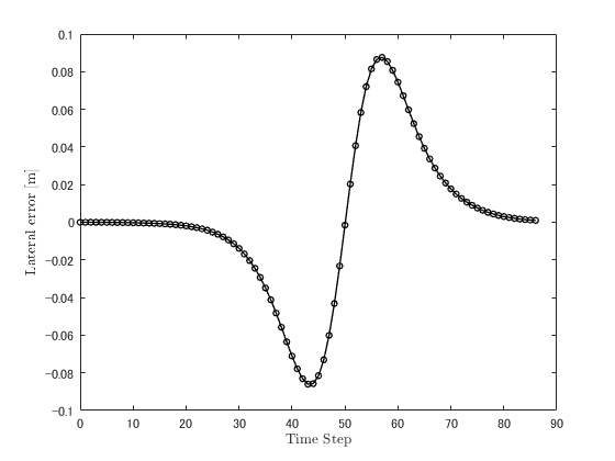
上記コードの実行結果を以下に示します.

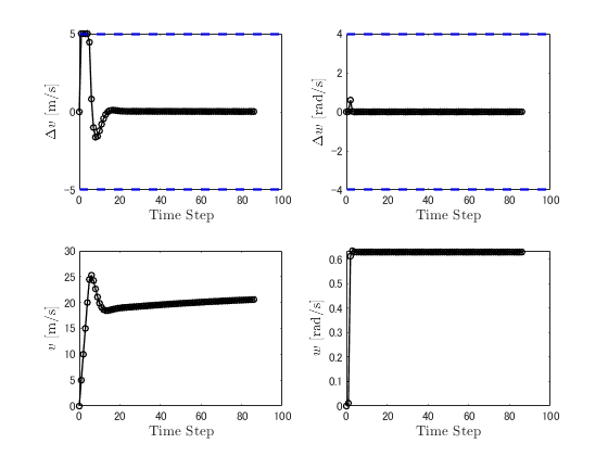

上記同様,軌道追従制御自体は出来ていますね. 最適制御問題の平均計算時間については,約0.0061秒と爆速で解いてますね(*゚∀゚)アヒャヒャ リアルタイム性に関しては全く問題ないですね!\(^o^)/
おわりに
今回は,モデル予測制御の最適制御問題を二次計画法で扱える形まで変形し,その効果を数値シミュレーションを通じて体感しました.少し数式をこねくり回して,二次計画法に帰着させるだけで,こんなに計算時間が向上するとは...
数学って本当大事だね( ´,_ゝ`)
参考文献
2.Vehicle Dynamics and Control, 2nd Edition