ニュートン法に基づく非線形モデル予測制御:MATLABサンプルプログラム
目次
はじめに
これまで,線形モデル,もしくは非線形モデルを線形化してモデル予測制御への適用について考えてきたわけですが...線形制御にはいくつか問題があります(TдT)
代表的な問題点として,実際の制御対象と物理モデルとの誤差が大きくなることが原因で制御がうまくできない場合が挙げられます.例えば,自動車の車線変更制御や障害物回避制御の場合,線形モデルだと実際の車両の運動と大きく異なるので,実世界での制御が難しいという問題が発生します.この課題の解決策の一つとして,非線形制御が挙げられます!
ここでは,非線形制御の内,非線形モデル予測制御についてまとめます. 非線形モデル予測制御については,過去にも素晴らしい記事がいくつかあるので,是非参照してみてください(*´ー`)
特に,大塚先生の「非線形モデル予測制御の研究動向」は是非目を通してみてくださいヽ(#゚Д゚)ノ!
https://www.jstage.jst.go.jp/article/isciesci/61/2/61_42/_pdf
非線形モデル予測制御について
ここでは,大塚先生の「実時間最適化による機械システムのモデル予測制御」,「実時間最適化による制御の実応用」を下に,非線形モデル予測制御について簡単にまとめます!
http://www2.iee.or.jp/~dmec/committee/DMEC8005/presentations/MCHF-4_ohtsuka.pdf
まず,モデル予測制御とは,各時刻で有限時間未来までの最適制御問題を解いて制御入力を決定しているフィードバック制御です.これを数式ベースで説明すると,以下のように定式化されます.
上記の最適制御問題は,上から順に非線形状態方程式,評価関数,制約条件を意味します. モデル予測制御では,各時刻で求めた最適制御を全て使うのではなく,初期値のみ使用します!←ここ重要(#゚Д゚)ゴルァ!!
さらに,求める最適制御と実際の制御入力の関係性を明らかにするために,現実の時刻とは別に評価区間上の時間軸
を新たに導入し,
時刻
をパラメータとみなして,
軸上で最適制御を求める手法がよくとられます.まとめると,時刻
で解くべき最適制御問題は,次のようになります!
このときの最適制御問題の停留条件は,以下のオイラー・ラグランジュ方程式によって与えられます.
ここで,
はハミルトン関数と呼ばれるものです.さらに,は随伴変数と呼ばれるベクトル,
は制約条件
に対するラグランジュ乗数のベクトルです.
オイラー・ラグランジュ方程式(´・ω・`) ?ナニソレ...となりませんか?←私はなりました(ノд`)
一言で片づけてしまうと,オイラー・ラグランジュ方程式は一般的な非線形最適制御問題の停留条件(KKT条件)であるわけですが,導出過程及び詳細については以下の文献の第3章,第5章あたりを参照してください.←投げま~す┐(´~`;)┌ www.coronasha.co.jp
ここでは,オイラー・ラグランジュ方程式について以下のポイントを押さえて頂ければいいと思います!
1については先ほど説明した通りですが,2についてはオイラー・ラグランジュ方程式より明らかです.オイラー・ラグランジュ方程式をよく観察すると,に対して初期条件を与え,
に対して終端条件を与えていることが分かります!このように,初期条件と終端条件の両方で境界条件が与えられている方程式を二点境界値問題と呼びます.二点境界値問題は状態方程式などが非線形な場合,一般的に解析的に解くのが困難となります.そのため,勾配法やニュートン法などの反復法から数値解を得るといったアプローチがよくとられます.つまり,毎時刻以下に示す手順により近似解を取得することになるわけです.
1.システムの状態を計測する .
2. を初期状態とした場合のオイラー・ラグランジュ方程式を勾配法やニュートン法で数値的に解いて,求めた最適制御の最初の要素を取得し,制御入力としてシステムに加える.
上記の処理を繰り返すことで,所望の目的を達成するための制御入力を求めます!
ニュートン法による非線形モデル予測制御の数値解法
ここでは,オイラー・ラグランジュ方程式を数値計算に適した問題で近似式に置き換えます.まず,評価区間をNステップに離散化し,時間刻みを
とします.このとき,オイラー・ラグランジュ方程式の内,状態と随伴変数に関する微分方程式を差分近似することで,以下の離散時間二点境界値問題を得ることが出来ます!
これは,状態の系列,制御入力の系列,随伴変数の系列,ラグランジュ乗数の系列に対する連立代数方程式と見なすことが出来るわけですが・・・以下のテクニカルな処理により,本質的な未知量は制御入力の系列とラグランジュ乗数の系列だけであることが分かります!
まず,制御入力とラグランジュ乗数からなるベクトルを定義します.
すると,オイラー・ラグランジュ方程式の状態方程式から状態の系列が求まり,それに付随して随伴変数の方程式からも随伴変数の系列が求まることが分かります.最後にオイラー・ラグランジュ方程式の内,残る条件式は以下の二つとなります.
このとき,これらの条件式は,
,
に依存しているため,離散時間二点境界値問題は
という代数方程式として表すことが出来ます( -ω- `)フッ
非線形モデル予測制御では,毎時刻上記の代数方程式の解を求め,その最初の要素を実際の制御入力として用います!
この代数方程式を解く際に,ニュートン法などの反復法を使用して数値解を取得するわけです!
ニュートン法については,以下の記事を是非参照してみてください (・∀・)
数値シミュレーション
さて,数式だけ眺めていても具体的な効果や実装面でイメージがつかないため,ここでは簡単な例題を通じて非線形モデル予測制御を体感してみましょう.
Case Study 1 : セミアクティブダンパの制御
以下の素晴らしい論文を参考に,モデル予測制御の数値シミュレーションをMATLABにより実装します. www.semanticscholar.org
制御対象のセミアクティブダンパの図を示します.

また,セミアクティブダンパの数理モデルは以下で定義されます.
ここで,状態量は2つあり,y方向の位置,y方向の速度,制御入力
は減衰係数です.また,入力に対して以下の不等式制約を与えます.
このとき,ダミー入力を導入することで,上記の不等式制約を以下の等式制約に変換することが出来ます.
さらに,評価関数を以下のように設定します.
ここで,評価関数の第一項目が終端コスト,第二項目がステージコスト
です.
今回の制御目的は,減衰係数を制御することで,全ての状態量を0に収束させることです.
下記がセミアクティブダンパの制御のMATLABコードになります.
clear;
close all;
clc;

%% Setup and Parameters
dt   = 0.01; % sample time
dimx = 2;    % Number of states
dimu = 3;    % Number of input(u1 = Attenuation coefficient, u2 = Dummy input, u3 = Lagrange multiplier)
diml = 2;    % Number of companion variable

sim_time = 20; % Simulation time [s]

%% Semi active dumper
system.m = 1; %[kg]
system.k = 1; %[N/m]
system.a = - system.k / system.m;
system.b = - 1 / system.m;

%% NMPC parameters
params_nmpc.tf = 1.0;             % Final value of prediction time [s]
params_nmpc.N = 5;                % Number of divisions of the prediction time [-]
params_nmpc.kmax = 20;            % Number of Newton's method
params_nmpc.hdir = 0.01;          % step in the Forward Difference Approximation

params_nmpc.x0 = [2;0];           % Initial state
params_nmpc.u0 = [0.01;0.9;0.03]; % Initial u

params_nmpc.sf = [ 1;10 ];        % Termination cost weight matrix
params_nmpc.q = [ 1;10 ];         % Weight matrix of state quantities
params_nmpc.r = [ 1;0.01 ];       % Weight matrix of input quantities

params_nmpc.umin = 0;             % lower input limit
params_nmpc.umax = 1;             % upper input limit

params_nmpc.dimx = dimx;          % Number of states
params_nmpc.dimu = dimu;          % Number of input(u1 = Attenuation coefficient, u2 = Dummy input, u3 = Lagrange multiplier)
params_nmpc.diml = diml;          % Number of companion variable

%% define systems
[xv, lmdv, uv, muv, fxu, Cxu] = defineSystem(system, params_nmpc);
[L, phi, qv, rv, sfv]         = evaluationFunction(xv, uv);
[obj, H, Hx, Hu, Huu, phix]   = generate_Euler_Lagrange_Equations(xv, lmdv, uv, muv, fxu, Cxu, L, phi, qv, rv, sfv);

%% Initial input value calculation using Newton's method
lmd0 = obj.phix(params_nmpc.x0, params_nmpc.sf);

for cnt = 1:params_nmpc.kmax
    params_nmpc.u0 = params_nmpc.u0 - obj.Huu( params_nmpc.u0, params_nmpc.r ) \ obj.Hu( params_nmpc.x0, params_nmpc.u0, lmd0, params_nmpc.r );
end

%% main loop
xTrue(:, 1) = params_nmpc.x0;
uk(:, 1) = params_nmpc.u0;
uk_horizon(:, 1) = repmat( params_nmpc.u0, params_nmpc.N, 1 );
current_step = 1;
sim_length = length(1:dt:sim_time);
normF = zeros(1, sim_length + 1);
solvetime = zeros(1, sim_length + 1);

for i = 1:dt:sim_time
    i
    % update time
    current_step = current_step + 1;

    % solve nmpc
    tic;
    [uk(:, current_step), uk_horizon(:, current_step), algebraic_equation] = NMPC( obj, xTrue(:, current_step - 1), uk_horizon(:, current_step - 1), system, params_nmpc);
    solvetime(1, current_step - 1) = toc;

    % optimality error norm F
    total = 0;
    for j = 1:params_nmpc.dimu * params_nmpc.N
        total = total + algebraic_equation(j, :)^2;
    end
    normF(1, current_step - 1) = sqrt(total);

    % update state
    T = dt*current_step:dt:dt*current_step+dt;
    [T, x] = ode45(@(t,x) nonlinear_model(x, uk(:, current_step), system), T, xTrue(:, current_step - 1));
    xTrue(:, current_step) = x(end,:);
end

%% solve average time
avg_time = sum(solvetime) / current_step;
disp(avg_time);

plot_figure(xTrue, uk, normF, current_step);

%% define systems
function [xv, lmdv, uv, muv, fxu, Cxu] = defineSystem(system, nmpc)
    syms x1 x2 lmd1 lmd2 u1 u2 u3
    xv   = [x1; x2];     % state vector
    lmdv = [lmd1; lmd2]; % costate vector
    uv   = [u1; u2];     % control input(include dummy input)
    muv  = u3;           % Lagrange multiplier vectors for equality constraints

    % state equation
    fxu = [xv(2);
           system.a * xv(1) + system.b* xv(2) * uv(1)];
    % constraints
    Cxu = (uv(1) - nmpc.umax / 2)^2 + uv(2)^2 - (nmpc.umax / 2)^2;
end

function [L, phi, qv, rv, sfv] = evaluationFunction(xv, uv)
    syms q1 q2 r1 r2 sf1 sf2
    qv  = [q1; q2];         % vector for diagonal matrix Q
    rv  = [r1; r2];         % weight vector
    sfv = [sf1; sf2];       % vector for diagonal matrix Sf
    Q   = diag([q1, q2]);   % square matrix
    R   = diag([r1, r2]);   % square matrix
    Sf  = diag([sf1, sf2]); % square matrix

    % stage cost
    L   = simplify( (xv' * Q * xv) / 2 + rv(1) * uv(1)^2 / 2 - rv(2) * uv(2) );
    % terminal cost
    phi = simplify( (xv' * Sf * xv) / 2 );
end

function [obj, H, Hx, Hu, Huu, phix] = generate_Euler_Lagrange_Equations(xv, lmdv, uv, muv, fxu, Cxu, L, phi, qv, rv, sfv)
    H = simplify(L + lmdv' * fxu + muv' * Cxu); % H = Hamiltonian
    uv = [uv; muv];                             % extend input

    Hx   = simplify(gradient(H, xv));           % Hx = ∂H / ∂x
    Hu   = simplify(gradient(H, uv));           % Hu = ∂H / ∂u
    Huu  = simplify(jacobian(Hu, uv));          % Huu = ∂^2H / ∂u^2
    phix = simplify(gradient(phi, xv));         % Huu = ∂φ / ∂x

    obj.Hx   = matlabFunction(Hx, 'vars', {xv, uv, lmdv, qv});
    obj.Hu   = matlabFunction(Hu, 'vars', {xv, uv, lmdv, rv});
    obj.Huu  = matlabFunction(Huu, 'vars', {uv, rv});
    obj.phix = matlabFunction(phix, 'vars', {xv, sfv});
end

%% NMPC
function [uk, uk_horizon, algebraic_equation] = NMPC( obj, x_current, uk_horizon, system, nmpc )
    for cnt = 1:nmpc.kmax
        uk_horizon = uk_horizon - ( dFdu( obj, x_current, uk_horizon, system, nmpc ) \ F( obj, x_current, uk_horizon, system, nmpc ) );
    end

    algebraic_equation = F( obj, x_current, uk_horizon, system, nmpc );
    uk = uk_horizon(1:nmpc.dimu);
end

%% calculation dF = ∂F / ∂u
function dF = dFdu( obj, x_current, u, system, nmpc )
    dF = zeros( nmpc.dimu * nmpc.N, nmpc.dimu * nmpc.N );
    diff = nmpc.hdir;

    for cnt = 1:nmpc.N*nmpc.dimu
        u_buff_p = u;
        u_buff_n = u;

        u_buff_p(cnt) = u_buff_p(cnt) + diff;
        u_buff_n(cnt) = u_buff_n(cnt) - diff;

        % dF = ∂F / ∂u is the Forward Difference Approximation
        dF(:,cnt) = ( F( obj, x_current, u_buff_p, system, nmpc ) - F( obj, x_current, u_buff_n, system, nmpc ) ) / ( diff );
    end
end

%% calculation F = nonlinear algebraic equation
function ans_F = F( obj, x_current, u, system, nmpc )
    x   = Forward( x_current, u, system, nmpc );
    lmd = Backward( obj, x, u, nmpc );

    ans_F = zeros( nmpc.dimu * nmpc.N, 1 );

    for cnt = 1:nmpc.N
        ans_F((1:nmpc.dimu)+nmpc.dimu*(cnt-1)) = obj.Hu(x((1:nmpc.dimx)+nmpc.dimx*(cnt-1)), ...
                                                        u((1:nmpc.dimu)+nmpc.dimu*(cnt-1)), ...
                                                        lmd((1:nmpc.diml)+nmpc.diml*(cnt-1)),...
                                                        nmpc.r );
    end
end

%% Prediction of the state from the current time to T seconds in the future (Euler approximation)
function x = Forward( x0, u, system, nmpc )
    dt = nmpc.tf / nmpc.N;

    x = zeros( nmpc.dimx * nmpc.N, 1 );
    x(1:nmpc.dimx) = x0;

    for cnt = 1 : nmpc.N-1
       x((1:nmpc.dimx)+nmpc.dimx*(cnt)) = x((1:nmpc.dimx)+nmpc.dimx*(cnt-1)) ...
                                        + nonlinear_model( x((1:nmpc.dimx)+nmpc.dimx*(cnt-1)), u((1:nmpc.dimu)+nmpc.dimu*(cnt-1)), system ) * dt;
    end
end

%% Prediction of adjoint variables from current time to T seconds in the future (Euler approximation)
function lmd = Backward( obj, x, u, nmpc )
    dt = nmpc.tf / nmpc.N;

    lmd = zeros( nmpc.diml * nmpc.N, 1 );
    lmd((1:nmpc.diml)+nmpc.diml*(nmpc.N-1)) = obj.phix( x((1:nmpc.dimx)+nmpc.dimx*(nmpc.N-1)), nmpc.sf );

    for cnt = nmpc.N-1:-1:1
        lmd((1:nmpc.diml)+nmpc.diml*(cnt-1)) = lmd((1:nmpc.diml)+nmpc.diml*(cnt)) ...
                                             + obj.Hx( x((1:nmpc.dimx)+nmpc.dimx*(cnt)), u, lmd((1:nmpc.diml)+nmpc.diml*(cnt)), nmpc.q ) * dt;
    end
end

%% nonlinear state equation
function dx = nonlinear_model(xTrue, u, system)
    % dx = f( xTrue, u )
    dx = [xTrue(2);
          system.a * xTrue(1) + system.b * xTrue(2) * u(1)];
end

%% plot figure
function plot_figure(xTrue, uk, normF, current_step)
    % plot state
    figure(1)
    subplot(2, 1, 1)
    plot(0:current_step - 1, xTrue(1,:), 'ko-',...
        'LineWidth', 1.0, 'MarkerSize', 4);
    xlabel('Time Step','interpreter','latex','FontSize',10);
    ylabel('y [m]','interpreter','latex','FontSize',10);
    yline(0.0, '--r', 'LineWidth', 1.0);

    subplot(2, 1, 2)
    plot(0:current_step - 1, xTrue(2,:), 'ko-',...
        'LineWidth', 1.0, 'MarkerSize', 4);
    xlabel('Time Step','interpreter','latex','FontSize',10);
    ylabel('$\dot{y}$ [m/s]','interpreter','latex','FontSize',10);
    yline(0.0, '--r', 'LineWidth', 1.0);

    % plot input
    figure(2);
    subplot(2, 1, 1)
    plot(0:current_step - 1, uk(1,:), 'ko-',...
        'LineWidth', 1.0, 'MarkerSize', 4);
    xlabel('Time Step','interpreter','latex','FontSize',10);
    ylabel('Attenuation coefficient [N/(m/s)]','interpreter','latex','FontSize',10);
    subplot(2, 1, 2)
    plot(0:current_step - 1, uk(2,:), 'ko-',...
        'LineWidth', 1.0, 'MarkerSize', 4);
    xlabel('Time Step','interpreter','latex','FontSize',10);
    ylabel('dummy input $\upsilon$','interpreter','latex','FontSize',10);

    % plot Lagrange multiplier
    figure(3);
    plot(0:current_step - 1, uk(3,:), 'ko-',...
        'LineWidth', 1.0, 'MarkerSize', 4);
    xlabel('Time Step','interpreter','latex','FontSize',10);
    ylabel('Lagrange multiplier $\mu$','interpreter','latex','FontSize',10);

    % plot optimality error
    figure(4);
    plot(0:current_step - 1, normF(1,:), 'ko-',...
        'LineWidth', 1.0, 'MarkerSize', 4);
    xlabel('Time Step','interpreter','latex','FontSize',10);
    ylabel('optimality error norm','interpreter','latex','FontSize',10);
end
下記のGitHubリポジトリでも公開しています. github.com
さらに,上記コードの実行結果を以下に示します.


結果より,制御目的はおおむね達成できていると言えそうです!また,制御入力に関しても制約条件内に収まっていることが確認できますね~.最適性誤差Fに関しては,初期誤差はかなり大きいですが,それ以外の時刻では,0に近い値を取っています(図だと分かりにくいです・・・(T_T)). また最適制御問題の平均計算時間は0.03[s]でした.しかし,ここではサンプリング周期0.01[s]と設定しているため,サンプリング周期内で制御入力の更新が出来ず,実機への適用が難しいことが分かります.このように,ニュートン法などの反復法は,解が収束するまでの計算時間を見積もることが難しく,一定のサンプリング周期でのフィードバック制御には向いていません(´;ω;`)←これが本記事で一番言いたいこと!!!
Case Study 2 : ホバークラフトの位置制御
Case Study 1同様,以下の素晴らしい論文を参考に,モデル予測制御の数値シミュレーションをMATLABにより実装します. www.semanticscholar.org

ここで,状態量は6つあり,x方向の位置,y方向の位置,方位角,x方向の速度,y方向の速度,角速度です.また,制御入力
は2つあり,それぞれ左右の推力です.さらに,入力に対して以下の不等式制約を与えます.
このとき,ダミー入力を導入することで,上記の不等式制約を以下の等式制約に変換することが出来ます.
ただし,は以下の通り定義されます.
さらに,評価関数を以下のように設定します.
ここで,評価関数の第一項目が終端コスト,第二項目がステージコスト
です.
今回の制御目的は,左右の推力を制御することで,目標状態
へ全ての状態量を収束させることです.
下記がホバークラフトの位置制御のMATLABコードになります.
clear;
close all;
clc;

%% Setup and Parameters
dt   = 0.01; % sample time
dimx = 6;    % Number of states
dimu = 6;    % Number of input(u1 = thrust1, u2 = thrust1, u3 = dummy input, u4 = dummy input, u5 = Lagrange multiplier1, u6 = Lagrange multiplier2)
diml = 6;    % Number of companion variable

sim_time = 10; % Simulation time [s]
end_condition = 0.0005; % [m]

%% Hovercraft
system.M = 0.894;  % [kg]
system.I = 0.0125; % [kg・m^2]
system.r = 0.0485; % [m]

%% NMPC parameters
params_nmpc.tf = 1.0;                                         % Final value of prediction time [s]
params_nmpc.N = 10;                                           % Number of divisions of the prediction time [-]
params_nmpc.kmax = 20;                                        % Number of Newton's method
params_nmpc.hdir = 0.0001;                                    % step in the Forward Difference Approximation

params_nmpc.x0 = [ -0.25; 0.35; 0.0; 0.0; 0.0; 0.0 ];         % Initial state
params_nmpc.u0 = [ 0.2; 0.1; 0.2; 0.03; 0.01; 0.02 ];         % Initial u
params_nmpc.xf = [ 0.0; 0.0; 0.0; 0.0; 0.0; 0.0 ];            % target state

params_nmpc.sf = [ 10; 15; 0.1; 1; 1; 0.01 ];                 % Termination cost weight matrix
params_nmpc.q  = [ 10; 15; 0.1; 1; 1; 0.01 ];                 % Weight matrix of state quantities
params_nmpc.r  = [ 1; 1; 0.001; 0.001 ];                      % Weight matrix of input quantities
params_nmpc.ki = [ 0.28; 0.28 ];                              % Weight matrix of dummy input

params_nmpc.umin = -0.121;                                    % lower input limit [N]
params_nmpc.umax = 0.342;                                     % upper input limit [N]
params_nmpc.uavg = (params_nmpc.umax + params_nmpc.umin) / 2; % average input limit [N]

params_nmpc.dimx = dimx;                                      % Number of states
params_nmpc.dimu = dimu;                                      % Number of input(u1 = Attenuation coefficient, u2 = Dummy input, u3 = Lagrange multiplier)
params_nmpc.diml = diml;                                      % Number of companion variable

%% define systems
[xv, lmdv, uv, muv, fxu, Cxu] = defineSystem(system, params_nmpc);
[L, phi, qv, rv, kv, sfv]     = evaluationFunction(xv, uv, params_nmpc);
[obj, H, Hx, Hu, Huu, phix]   = generate_Euler_Lagrange_Equations(xv, lmdv, uv, muv, fxu, Cxu, L, phi, qv, rv, kv, sfv);

%% Initial input value calculation using Newton's method
lmd0 = obj.phix(params_nmpc.x0, params_nmpc.sf);

for cnt = 1:params_nmpc.kmax
    params_nmpc.u0 = params_nmpc.u0 - obj.Huu( params_nmpc.u0, params_nmpc.r ) \ obj.Hu( params_nmpc.x0, params_nmpc.u0, lmd0, params_nmpc.r, params_nmpc.ki );
end

%% main loop
xTrue(:, 1) = params_nmpc.x0;
uk(:, 1) = params_nmpc.u0;
uk_horizon(:, 1) = repmat( params_nmpc.u0, params_nmpc.N, 1 );
current_step = 1;
sim_length = length(1:dt:sim_time);
normF = zeros(1, sim_length + 1);
solvetime = zeros(1, sim_length + 1);

for i = 1:dt:sim_time
    i
    % update time
    current_step = current_step + 1;

    % solve nmpc
    tic;
    [uk(:, current_step), uk_horizon(:, current_step), algebraic_equation] = NMPC( obj, xTrue(:, current_step - 1), uk_horizon(:, current_step - 1), system, params_nmpc);
    solvetime(1, current_step - 1) = toc;

    % optimality error norm F
    total = 0;
    for j = 1:params_nmpc.dimu * params_nmpc.N
        total = total + algebraic_equation(j, :)^2;
    end
    normF(1, current_step - 1) = sqrt(total);

    % update state
    T = dt*current_step:dt:dt*current_step+dt;
    [T, x] = ode45(@(t,x) nonlinear_model(x, uk(:, current_step), system), T, xTrue(:, current_step - 1));
    xTrue(:, current_step) = x(end,:);

    % break condition
    x_target  = params_nmpc.xf;
    x_current = xTrue(:, current_step);
    if ( (x_current(1) - x_target(1))^2 + (x_current(2) - x_target(2))^2 ) <= end_condition
        break
    end
end

%% solve average time
avg_time = sum(solvetime) / current_step;
disp(avg_time);

plot_figure(xTrue, uk, normF, params_nmpc, current_step);

%% define systems
function [xv, lmdv, uv, muv, fxu, Cxu] = defineSystem(system, nmpc)
    syms x1 x2 x3 x4 x5 x6 lmd1 lmd2 lmd3 lmd4 lmd5 lmd6 u1 u2 u3 u4 u5 u6
    xv   = [x1; x2; x3; x4; x5; x6];             % state vector
    lmdv = [lmd1; lmd2; lmd3; lmd4; lmd5; lmd6]; % costate vector
    uv   = [u1; u2; u3; u4];                     % control input(include dummy input)
    muv  = [u5; u6];                             % Lagrange multiplier vectors for equality constraints

    % state equation
    fxu = [xv(4);
           xv(5);
           xv(6);
           ( uv(1) * cos(xv(3)) + uv(2) * cos(xv(3)) ) / system.M;
           ( uv(1) * sin(xv(3)) + uv(2) * sin(xv(3)) ) / system.M;
           ( uv(1) * system.r + uv(2) * system.r ) / system.I];
    % constraints
    Cxu = [(uv(1) - nmpc.uavg)^2 + uv(3)^2 - (nmpc.umax - nmpc.uavg)^2;
           (uv(2) - nmpc.uavg)^2 + uv(4)^2 - (nmpc.umax - nmpc.uavg)^2];
end

function [L, phi, qv, rv, kv, sfv] = evaluationFunction(xv, uv, nmpc)
    syms q1 q2 q3 q4 q5 q6 r1 r2 r3 r4 k1 k2 sf1 sf2 sf3 sf4 sf5 sf6
    qv  = [ q1; q2; q3; q4; q5; q6 ];           % vector for diagonal matrix Q
    rv  = [ r1; r2; r3; r4 ];                   % vector for diagonal matrix R
    kv  = [ k1; k2 ];                           % weight vector
    sfv = [ sf1; sf2; sf3; sf4; sf5; sf6 ];     % vector for diagonal matrix Sf
    Q   = diag([q1, q2, q3, q4, q5, q6]);       % square matrix
    R   = diag([r1, r2, r3, r4]);               % square matrix
    Sf  = diag([sf1, sf2, sf3, sf4, sf5, sf6]); % square matrix

    % stage cost
    L   = simplify( ((xv - nmpc.xf)' * Q * (xv - nmpc.xf)) / 2 + (uv' * R * uv) / 2 - kv(1) * uv(3) - kv(2) * uv(4) );
    % terminal cost
    phi = simplify( ((xv - nmpc.xf)' * Sf * (xv - nmpc.xf)) / 2 );
end

function [obj, H, Hx, Hu, Huu, phix] = generate_Euler_Lagrange_Equations(xv, lmdv, uv, muv, fxu, Cxu, L, phi, qv, rv, kv, sfv)
    H = simplify(L + lmdv' * fxu + muv' * Cxu); % H = Hamiltonian
    uv = [uv; muv];                             % extend input

    Hx   = simplify(gradient(H, xv));           % Hx = ∂H / ∂x
    Hu   = simplify(gradient(H, uv));           % Hu = ∂H / ∂u
    Huu  = simplify(jacobian(Hu, uv));          % Huu = ∂^2H / ∂u^2
    phix = simplify(gradient(phi, xv));         % Huu = ∂φ / ∂x

    obj.Hx   = matlabFunction(Hx, 'vars', {xv, uv, lmdv, qv});
    obj.Hu   = matlabFunction(Hu, 'vars', {xv, uv, lmdv, rv, kv});
    obj.Huu  = matlabFunction(Huu, 'vars', {uv, rv});
    obj.phix = matlabFunction(phix, 'vars', {xv, sfv});
end

%% NMPC
function [uk, uk_horizon, algebraic_equation] = NMPC( obj, x_current, uk_horizon, system, nmpc )
    for cnt = 1:nmpc.kmax
        uk_horizon = uk_horizon - ( dFdu( obj, x_current, uk_horizon, system, nmpc ) \ F( obj, x_current, uk_horizon, system, nmpc ) );
    end

    algebraic_equation = F( obj, x_current, uk_horizon, system, nmpc );
    uk = uk_horizon(1:nmpc.dimu);
end

%% calculation dF = ∂F / ∂u
function dF = dFdu( obj, x_current, u, system, nmpc )
    dF = zeros( nmpc.dimu * nmpc.N, nmpc.dimu * nmpc.N );
    diff = nmpc.hdir;

    for cnt = 1:nmpc.N*nmpc.dimu
        u_buff_p = u;
        u_buff_n = u;

        u_buff_p(cnt) = u_buff_p(cnt) + diff;
        u_buff_n(cnt) = u_buff_n(cnt) - diff;

        % dF = ∂F / ∂u is the Forward Difference Approximation
        dF(:,cnt) = ( F( obj, x_current, u_buff_p, system, nmpc ) - F( obj, x_current, u_buff_n, system, nmpc ) ) / ( diff );
    end
end

%% calculation F = nonlinear algebraic equation
function ans_F = F( obj, x_current, u, system, nmpc )
    x   = Forward( x_current, u, system, nmpc );
    lmd = Backward( obj, x, u, nmpc );

    ans_F = zeros( nmpc.dimu * nmpc.N, 1 );

    for cnt = 1:nmpc.N
        ans_F((1:nmpc.dimu)+nmpc.dimu*(cnt-1)) = obj.Hu(x((1:nmpc.dimx)+nmpc.dimx*(cnt-1)), ...
                                                        u((1:nmpc.dimu)+nmpc.dimu*(cnt-1)), ...
                                                        lmd((1:nmpc.diml)+nmpc.diml*(cnt-1)),...
                                                        nmpc.r,...
                                                        nmpc.ki);
    end
end

%% Prediction of the state from the current time to T seconds in the future (Euler approximation)
function x = Forward( x0, u, system, nmpc )
    dt = nmpc.tf / nmpc.N;

    x = zeros( nmpc.dimx * nmpc.N, 1 );
    x(1:nmpc.dimx) = x0;

    for cnt = 1 : nmpc.N-1
       x((1:nmpc.dimx)+nmpc.dimx*(cnt)) = x((1:nmpc.dimx)+nmpc.dimx*(cnt-1)) ...
                                        + nonlinear_model( x((1:nmpc.dimx)+nmpc.dimx*(cnt-1)), u((1:nmpc.dimu)+nmpc.dimu*(cnt-1)), system ) * dt;
    end
end

%% Prediction of adjoint variables from current time to T seconds in the future (Euler approximation)
function lmd = Backward( obj, x, u, nmpc )
    dt = nmpc.tf / nmpc.N;

    lmd = zeros( nmpc.diml * nmpc.N, 1 );
    lmd((1:nmpc.diml)+nmpc.diml*(nmpc.N-1)) = obj.phix( x((1:nmpc.dimx)+nmpc.dimx*(nmpc.N-1)), nmpc.sf );

    for cnt = nmpc.N-1:-1:1
        lmd((1:nmpc.diml)+nmpc.diml*(cnt-1)) = lmd((1:nmpc.diml)+nmpc.diml*(cnt)) ...
                                             + obj.Hx( x((1:nmpc.dimx)+nmpc.dimx*(cnt)), u, lmd((1:nmpc.diml)+nmpc.diml*(cnt)), nmpc.q ) * dt;
    end
end

%% nonlinear state equation
function dx = nonlinear_model(xTrue, u, system)
    % dx = f( xTrue, u )
    dx = [xTrue(4);
          xTrue(5);
          xTrue(6);
          ( u(1) * cos(xTrue(3)) + u(2) * cos(xTrue(3)) ) / system.M;
          ( u(1) * sin(xTrue(3)) + u(2) * sin(xTrue(3)) ) / system.M;
          ( u(1) * system.r + u(2) * system.r ) / system.I];
end

%% plot figure
function plot_figure(xTrue, uk, normF, nmpc, current_step)
    % plot state
    figure(1)
    subplot(3, 1, 1)
    plot(0:current_step - 1, xTrue(1,:), 'ko-',...
        'LineWidth', 1.0, 'MarkerSize', 4);
    xlabel('Time Step','interpreter','latex','FontSize',10);
    ylabel('X [m]','interpreter','latex','FontSize',10);
    yline(0.0, '--r', 'LineWidth', 2.0);

    subplot(3, 1, 2)
    plot(0:current_step - 1, xTrue(2,:), 'ko-',...
        'LineWidth', 1.0, 'MarkerSize', 4);
    xlabel('Time Step','interpreter','latex','FontSize',10);
    ylabel('Y [m]','interpreter','latex','FontSize',10);
    yline(0.0, '--r', 'LineWidth', 2.0);

    subplot(3, 1, 3)
    plot(0:current_step - 1, xTrue(3,:), 'ko-',...
        'LineWidth', 1.0, 'MarkerSize', 4);
    xlabel('Time Step','interpreter','latex','FontSize',10);
    ylabel('$\theta$ [rad]','interpreter','latex','FontSize',10);
    yline(0.0, '--r', 'LineWidth', 2.0);

    % plot state
    figure(2);
    subplot(3, 1, 1)
    plot(0:current_step - 1, xTrue(4,:), 'ko-',...
        'LineWidth', 1.0, 'MarkerSize', 4);
    xlabel('Time Step','interpreter','latex','FontSize',10);
    ylabel('$\dot{X}$ [m/s]','interpreter','latex','FontSize',10);
    yline(0.0, '--r', 'LineWidth', 2.0);

    subplot(3, 1, 2)
    plot(0:current_step - 1, xTrue(5,:), 'ko-',...
        'LineWidth', 1.0, 'MarkerSize', 4);
    xlabel('Time Step','interpreter','latex','FontSize',10);
    ylabel('$\dot{Y}$ [m/s]','interpreter','latex','FontSize',10);
    yline(0.0, '--r', 'LineWidth', 2.0);

    subplot(3, 1, 3)
    plot(0:current_step - 1, xTrue(6,:), 'ko-',...
        'LineWidth', 1.0, 'MarkerSize', 4);
    xlabel('Time Step','interpreter','latex','FontSize',10);
    ylabel('$\dot{\theta}$ [rad/s]','interpreter','latex','FontSize',10);
    yline(0.0, '--r', 'LineWidth', 2.0);

    % plot input
    figure(3);
    subplot(2, 1, 1)
    plot(0:current_step - 1, uk(1,:), 'ko-',...
        'LineWidth', 1.0, 'MarkerSize', 4);
    xlabel('Time Step','interpreter','latex','FontSize',10);
    ylabel('$u_{1}$ [N]','interpreter','latex','FontSize',10);
    yline(nmpc.umin, '--b', 'LineWidth', 2.0);
    yline(nmpc.umax, '--b', 'LineWidth', 2.0);

    subplot(2, 1, 2)
    plot(0:current_step - 1, uk(2,:), 'ko-',...
        'LineWidth', 1.0, 'MarkerSize', 4);
    xlabel('Time Step','interpreter','latex','FontSize',10);
    ylabel('$u_{2}$ [N]','interpreter','latex','FontSize',10);
    yline(nmpc.umin, '--b', 'LineWidth', 2.0);
    yline(nmpc.umax, '--b', 'LineWidth', 2.0);

    % plot dummy input
    figure(4);
    subplot(2, 1, 1)
    plot(0:current_step - 1, uk(3,:), 'ko-',...
        'LineWidth', 1.0, 'MarkerSize', 4);
    xlabel('Time Step','interpreter','latex','FontSize',10);
    ylabel('dummy input $u_{d1}$','interpreter','latex','FontSize',10);
    subplot(2, 1, 2)
    plot(0:current_step - 1, uk(4,:), 'ko-',...
        'LineWidth', 1.0, 'MarkerSize', 4);
    xlabel('Time Step','interpreter','latex','FontSize',10);
    ylabel('dummy input $u_{d2}$','interpreter','latex','FontSize',10);

    % plot Lagrange multiplier
    figure(5);
    subplot(2, 1, 1)
    plot(0:current_step - 1, uk(5,:), 'ko-',...
        'LineWidth', 1.0, 'MarkerSize', 4);
    xlabel('Time Step','interpreter','latex','FontSize',10);
    ylabel('Lagrange multiplier $\mu_{1}$','interpreter','latex','FontSize',10);
    subplot(2, 1, 2)
    plot(0:current_step - 1, uk(6,:), 'ko-',...
        'LineWidth', 1.0, 'MarkerSize', 4);
    xlabel('Time Step','interpreter','latex','FontSize',10);
    ylabel('Lagrange multiplier $\mu_{2}$','interpreter','latex','FontSize',10);

    % plot optimality error
    figure(6);
    plot(0:current_step - 1, normF(1,1:current_step), 'ko-',...
        'LineWidth', 1.0, 'MarkerSize', 4);
    xlabel('Time Step','interpreter','latex','FontSize',10);
    ylabel('optimality error norm F','interpreter','latex','FontSize',10);

    % plot trajectory
    figure(7)
    plot(xTrue(1,:), xTrue(2,:), 'b',...
        'LineWidth', 2.0, 'MarkerSize', 4); hold on;
    grid on;
    % plot target position
    target = nmpc.xf;
    plot(target(1), target(2), 'dg', 'LineWidth', 2);
    xlabel('X [m]','interpreter','latex','FontSize',10);
    ylabel('Y [m]','interpreter','latex','FontSize',10);
    legend('Motion trajectory', 'Target position', 'Location','southeast',...
           'interpreter','latex','FontSize',10.0);
end
下記のGitHubリポジトリでも公開しています. github.com
さらに,上記コードの実行結果を以下に示します.


結果より,初期位置から目的地までおおむね到達できていることが確認できます!また,制御入力に関しても制約条件内に収まっていることが確認できますね~.最適性誤差Fに関しても初期値含め,0に近い状態を保っていることが分かります. また最適制御問題の平均計算時間は0.65[s]と,サンプリング周期0.01[s]に比べて大幅に時間が掛かっていることが分かりました.Case Study 1に比べて制御入力が増加したこと,状態量が増加したこと,非線形性が増したことなど様々な理由により,処理負荷が増加したのだと思います.
まとめ
ここでは,一般的な非線形モデル予測制御の定式化及び最適性条件である代数方程式の簡単な流れと数値シミュレーション例についてまとめました.代数方程式の解を得るためにここではニュートン法を使用して数値解を取得したわけですが,案の定ニュートン法などの反復法では計算時間がかかり(正確にはサンプリング周期内では解けず)実機への適用は難しいことが確認できました(ˇ・ω・ˇ)
この代数方程式を高速で解くための研究というのはいくつかなされているそうですが,その中でも最も有名な手法がC/GMRES法だと思います.C/GMRES法に基づく非線形モデル予測制御についてもまとめたい\(^o^)/
参考文献
二次計画法に基づく線形モデル予測制御による軌道追従制御:MATLABサンプルプログラム
目次
はじめに
以前,線形モデル予測制御について以下の記事でまとめましたが,やはりリアルタイム性の面で問題があることが分かりました(T_T)
上記の記事では,評価関数をステージコストと終端コストの和として考え,最適制御問題の定式化を行いました.ただし,これはあくまでモデル予測制御の表現方法の一つでしかなく,他にも様々な表現方法があります!その内の一つに,最適制御問題を二次計画問題に落とし込むというものがあります.先に結論を言ってしまうと,この二次計画法,リアルタイム性がめちゃくちゃあるんです!一番の理由は,「評価関数が決定変数に対して下に凸な二次関数のため,最適解を求めることが容易」だからです!凸とは何ぞや?という方は以下の素晴らしい記事で解説されているので是非参考にしてください.
より本格的に凸最適化問題について学びたい場合は,以下の参考書(Convex Optimization)が最も詳しく書かれていると思います.
https://web.stanford.edu/~boyd/cvxbook/bv_cvxbook.pdf
私も5章ぐらいまで読みましたが,挫折しました...(´・ω・`) PDFファイルが無料で配布されているので是非!
ここでは簡単に,凸関数の概念について説明します.まず,下に凸な二次関数とは具体的には,以下の図のようなものを指します.

このとき,決定変数が]の場合,評価関数を最小化する
と
の組は容易に求めることが可能なのは直感的にも分かると思います!
二次計画法では評価関数をこのような関数の形に変形してから,予測ホライズン分の最適解を一気に求めるため計算時間が早いわけです.←ここ重要(_)
それでは,具体的にどのように変形していくのか,また実際どの程度リアルタイム性があるのか,軌道追従問題を題材に順を追って確認していきましょう!
二次計画法に基づく線形モデル予測制御の定式化
まず,扱う制御対象のシステムを定義します.
上記の線形モデルに対して,最適制御問題では以下のような評価関数を設定していました.
ここで,第一項目が終端コスト,第二項目がステージコストです.本来はこれに加えていくつかの制約条件を考慮して解きます.このとき,上記の評価関数は平衡点,つまり状態量を0に収束させるような評価指標になっていますが,実際は何かしらの制御目標値に到達することを考えます.そのため,一般的には以下の評価関数を考えることが多いです.
ここで,
と定義します.このとき,は目標値で,
は状態の観測値です.つまり,目標値と現在の状態との偏差を最小化する制御入力を求める問題というわけです.本記事では,この目標値を参照軌道とします.
ここで,参照軌道に追従し続けるには,入力が常に0ではなく何かしらの値を保持している必要があります.しかし,上記の評価関数だと状態量が目標値に到達すれば,制御対象は安定となるため,入力の変化量が0になります.したがって,軌道追従問題では,入力の変化量を使用して,入力値を以下にように定義します.
同時に,制御対象は以下のように書きかえることが出来ます.
このとき,[tex: x{k+1} ]は過去の入力値[tex: u{k+1} ]に依存していることに注意します.このような場合,過去の入力値も状態量に加えた形で状態方程式を拡張します.
上記の拡張状態方程式と入力の変化量に対して,評価関数を以下のように書き直します.
さらに,上記の評価関数を以下のように展開します.
ここまでは,終端コストとステージコストを分けて表現する方法になっています.ここから,二次計画法の形に落とし込むために,以下のように時系列順に状態量を並べたベクトルを定義します.
状態量をこのように表現することで,Σの足し合わせの項をベクトル表記で一気に記述することが可能となります.(いきなり,以下の数式が出てきて戸惑う方もいるかもしれません.その場合は,一度行列の四則演算に従って展開してみることをおすすめします.展開計算をすることで,Σの足し合わせに相当していることが確認できます.)
割とすっきりした形になりましたね(*゚∀゚)アヒャヒャ
これで終わりかと思いきや,まだやることがあります.上記の評価関数は拡張状態量と入力の変化量との二変数関数となっており,このままでは二次計画法を利用できません.ここで改めて制御の目的を振り返ると...目標値へ追従しつづけるために必要な入力の変化量[tex: \Delta u{k} ]を求めることです!!!
つまり,二次計画法の決定変数を入力の変化量[tex: \Delta u{k} ]に統一した形にもっていきたいわけです!←ここ重要ヾ(゚Д゚)ノ.
そのためには,余計な変数に消えてもらわなくてはいけませんね~.それは拡張状態量です!
では,にどのように消えてもらえばいいのでしょうか?
答えは単純で,
を
で表現出来ればいいわけです.
では,
は具体的にどのように記述できるのか?ここで,拡張状態量の各時系列要素は以下のように更新されていきます.
上記の数式の羅列をよく観察すると,拡張状態量が以下の数式でまとめることが出来ることに気づきます←最初,私は気づきませんでした( ᷄・‸・᷅ )
さて,拡張状態量を
に依存した形に落とし込めたので,これを先ほど導出した二変数関数に代入しましょう!
上記の評価関数の内,入力の変化量に関する項以外は全て定数項となるため無視すと,最終的に以下の数式にたどり着きます.←(ここも基本的には,数式展開を行って整理するだけです!)
これで,評価関数が入力の変化量の二次形式になりました!う~ん,長かったですがこれで変形部分は終わりです\(^o^)/オワタ
実際には,上記の二次計画問題を制御周期毎に解き,その最初の要素を実際の制御対象へ印加するという流れになります.
数値シミュレーション
さて,数式だけ眺めていても具体的な効果や実装面のイメージがつかないため,ここでは簡単な例題を通じてモデル予測制御に基づく軌道追従制御を体感してみましょう.
Case Study 1:自動車の軌道追従制御

まずは,以下の資料を参考に,自動車の軌道追従制御を行います.
自動車の数理モデルは以下の式で記述されます.
ここでは,車両速度は一定とし,自動車の舵角(正確には舵角の変化量)を制御することで,与えた参照軌道への追従制御を考えます.
また,二次計画法のリアルタイム性を検証するために,以下の定式化に基づくモデル予測制御との比較を行います.
これは,以前の記事でも何パターンかの制御対象と問題設定で検証しましたが,そこまでリアルタイム性のある結果を得ることが出来なかった定式化です.詳細については,以下の記事をどうぞ ( ^ω^)
上記定式化に基づく自動車の軌道追従制御のMATLABコードを以下に示します. また,ソルバーはYALMIPのIPOPTを使用しています.
clear;
close all;
clc;

%% Ipopt solver path
dir = pwd;
addpath(fullfile(dir,'Ipopt'))

%% Choice the type of trajectory
while true
    model = input('Please choose the type of trajectory (1 = Lane change, 2 = Circle): ');
    switch model
        case 1
            trajectory_type = 'Lane change';
            break;
        case 2
            trajectory_type = 'Circle';
            break;
        otherwise
            disp('No System!');
    end
end

%% Setup and Parameters
dt = 0.1; % sample time
nx = 4;   % Number of states
ny = 2;   % Number of ovservation
nu = 1;   % Number of input

S = diag([10.0, 1.0]); % Termination cost weight matrix
Q = diag([10.0, 1.0]); % Weight matrix of state quantities
R = 30.0;              % Weight matrix of input quantities
N = 15;                % Predictive Horizon

% Range of inputs
umin = -pi / 60;
umax = pi / 60;

%% Linear Car models (Lateral Vehicle Dynamics)
M = 1500;     % [kg]
I = 3000;     % [kgm^2]
lf = 1.2;     % [m]
lr = 1.6;     % [m]
l = lf + lr;  % [m]
Kf = 19000;   % [N/rad]
Kr = 33000;   % [N/rad]
Vx = 20;      % [m/s]

system.dt = dt;
system.nx = nx;
system.ny = ny;
system.nu = nu;

% states = [y_dot, psi, psi_dot, Y];
% Vehicle Dynamics and Control (2nd edition) by Rajesh Rajamani. They are in Chapter 2.3.
A11 = -2 * (Kf + Kr)/(M * Vx);
A13 = -Vx - 2 * (Kf*lf - Kr*lr)/(M * Vx);
A31 = -2 * (lf*Kf - lr*Kr)/(I * Vx);
A33 = -2 * (lf^2*Kf + lr^2*Kr)/(I * Vx);
system.A = eye(nx) + [A11, 0.0, A13, 0.0;
                      0.0, 0.0, 1.0, 0.0;
                      A31, 0.0, A33, 0.0;
                      1.0, Vx, 0.0, 0.0] * dt;

B11 = 2*Kf/M;
B13 = 2*lf*Kf/I;
system.B = [B11;
            0.0;
            B13;
            0.0] * dt;

system.C = [0 1 0 0;
            0 0 0 1];

system.A_aug = [system.A, system.B;
                zeros(length(system.B(1,:)),length(system.A(1,:))),eye(length(system.B(1,:)))];
system.B_aug = [system.B;
                eye(length(system.B(1,:)))];
system.C_aug = [system.C,zeros(length(system.C(:,1)),length(system.B(1,:)))];

% Constants
system.Vx = Vx;
system.M  = M;
system.I  = I;
system.Kf = Kf;
system.Kr = Kr;
system.lf = lf;
system.lr = lr;

% input
system.ul = umin;
system.uu = umax;

%% Load the trajectory
if strcmp(trajectory_type, 'Lane change')
    t = 0:dt:10.0;
elseif strcmp(trajectory_type, 'Circle')
    t = 0:dt:80.0;
end
[x_ref, y_ref, psi_ref] = trajectory_generator(t, Vx, trajectory_type);

sim_length = length(t); % Number of control loop iterations

refSignals = zeros(length(x_ref(:, 1)) * ny, 1);

ref_index = 1;
for i = 1:ny:length(refSignals)
    refSignals(i)     = psi_ref(ref_index, 1);
    refSignals(i + 1) = y_ref(ref_index, 1);
    ref_index = ref_index + 1;
end

% initial state
x0 = [0.0; psi_ref(1, 1); 0.0; y_ref(1, 1)]; % Initial state of Lateral Vehicle Dynamics

%% MPC parameters
params_mpc.Q = Q;
params_mpc.R = R;
params_mpc.S = S;
params_mpc.N = N;

%% main loop
xTrue(:, 1) = x0;
uk(:, 1) = 0.0;
du(:, 1) = 0.0;
current_step = 1;
solvetime = zeros(1, sim_length);

ref_sig_num = 1; % for reading reference signals
for i = 1:sim_length-15
    % update time
    current_step = current_step + 1;

    % Generating the current state and the reference vector
    xTrue_aug = [xTrue(:, current_step - 1); uk(:, current_step - 1)];
    ref_sig_num = ref_sig_num + ny;

    if ref_sig_num + ny * N - 1 <= length(refSignals)
        ref = refSignals(ref_sig_num:ref_sig_num+ny*N-1);
    else
        ref = refSignals(ref_sig_num:length(refSignals));
        N = N - 1;
    end

    % solve mac
    tic;
    du(:, current_step) = mpc(xTrue_aug, system, params_mpc, ref);
    solvetime(1, current_step - 1) = toc;

    % add du input
    uk(:, current_step) = uk(:, current_step - 1) + du(:, current_step);

    % update state
    T = dt*i:dt:dt*i+dt;
    [T, x] = ode45(@(t,x) nonlinear_lateral_car_model(t, x, uk(:, current_step), system), T, xTrue(:, current_step - 1));
    xTrue(:, current_step) = x(end,:);
end

%% solve average time
avg_time = sum(solvetime) / current_step;
disp(avg_time);

drow_figure(xTrue, uk, du, x_ref, y_ref, current_step, trajectory_type);

%% model predictive control
function uopt = mpc(xTrue_aug, system, params, ref)
    % Solve MPC
    [feas, ~, u, ~] = solve_mpc(xTrue_aug, system, params, ref);
    if ~feas
        uopt = [];
        return
    else
        uopt = u(:, 1);
    end
end

function [feas, xopt, uopt, Jopt] = solve_mpc(xTrue_aug, system, params, ref)
    % extract variables
    N = params.N;
    % define variables and cost
    x = sdpvar(system.nx + system.nu, N+1);
    u = sdpvar(system.nu, N);
    constraints = [];
    cost = 0;
    ref_index = 1;

    % initial constraint
    constraints = [constraints; x(:,1) == xTrue_aug];
    % add constraints and costs
    for i = 1:N-1
        constraints = [constraints;
            system.ul <= u(:,i) <= system.uu
            x(:,i+1) == system.A_aug * x(:,i) + system.B_aug * u(:,i)];
        cost = cost + (ref(ref_index:ref_index + 1,1) - system.C_aug * x(:,i+1))' * params.Q * (ref(ref_index:ref_index + 1,1) - system.C_aug * x(:,i+1)) + u(:,i)' * params.R * u(:,i);
        ref_index = ref_index + system.ny;
    end
    % add terminal cost
    cost = cost + (ref(ref_index:ref_index+1,1) - system.C_aug * x(:,N+1))' * params.S * (ref(ref_index:ref_index+1,1) - system.C_aug * x(:,N+1));
    ops = sdpsettings('solver','ipopt','verbose',0);
    % solve optimization
    diagnostics = optimize(constraints, cost, ops);
    if diagnostics.problem == 0
        feas = true;
        xopt = value(x);
        uopt = value(u);
        Jopt = value(cost);
    else
        feas = false;
        xopt = [];
        uopt = [];
        Jopt = [];
    end
end

%% trajectory generator
function [x_ref, y_ref, psi_ref] = trajectory_generator(t, Vx, trajectory_type)
    if strcmp(trajectory_type, 'Lane change')
        x = linspace(0, Vx * t(end), length(t));
        y = 3 * tanh((t - t(end) / 2));
    elseif strcmp(trajectory_type, 'Circle')
        radius = 30;
        period = 1000;
        for i = 1:length(t)
            x(1, i) = radius * sin(2 * pi * i / period);
            y(1, i) = -radius * cos(2 * pi * i / period);
        end
    end

    dx = x(2:end) - x(1:end-1);
    dy = y(2:end) - y(1:end-1);

    psi    = zeros(1,length(x));
    psiInt = psi;

    psi(1)     = atan2(dy(1),dx(1));
    psi(2:end) = atan2(dy(:),dx(:));
    dpsi       = psi(2:end) - psi(1:end-1);

    psiInt(1) = psi(1);
    for i = 2:length(psiInt)
        if dpsi(i - 1) < -pi
            psiInt(i) = psiInt(i - 1) + (dpsi(i - 1) + 2 * pi);
        elseif dpsi(i - 1) > pi
            psiInt(i) = psiInt(i - 1) + (dpsi(i - 1) - 2 * pi);
        else
            psiInt(i) = psiInt(i - 1) + dpsi(i - 1);
        end
    end

    x_ref   = x';
    y_ref   = y';
    psi_ref = psiInt';
end

function dx = nonlinear_lateral_car_model(t, xTrue, u, system)
    % In this simulation, the body frame and its transformation is used
    % instead of a hybrid frame. That is because for the solver ode45, it
    % is important to have the nonlinear system of equations in the first
    % order form.

    % Get the constants from the general pool of constants
    Vx = system.Vx;
    M  = system.M;
    I  = system.I;
    Kf = system.Kf;
    Kr = system.Kr;
    lf = system.lf;
    lr = system.lr;

    % % Assign the states
    y_dot   = xTrue(1);
    psi     = xTrue(2);
    psi_dot = xTrue(3);

    % The nonlinear equation describing the dynamics of the car
    dx(1,1) = -(2*Kf+2*Kr)/(M * Vx)*y_dot+(-Vx-(2*Kf*lf-2*Kr*lr)/(M * Vx))*psi_dot+2*Kf/M*u;
    dx(2,1) = psi_dot;
    dx(3,1) = -(2*lf*Kf-2*lr*Kr)/(I * Vx)*y_dot-(2*lf^2*Kf+2*lr^2*Kr)/(I * Vx)*psi_dot+2*lf*Kf/I*u;
    dx(4,1) = sin(psi) * Vx + cos(psi) * y_dot;
end

function drow_figure(xTrue, uk, du, x_ref, y_ref, current_step, trajectory_type)
    % Plot simulation
    figure(1)
    subplot(2, 1, 1)
    plot(0:current_step - 1, du(1,:), 'ko-',...
        'LineWidth', 1.0, 'MarkerSize', 4);
    xlabel('Time Step','interpreter','latex','FontSize',10);
    ylabel('$\Delta \delta$ [rad]','interpreter','latex','FontSize',10);
    yline(pi / 60, '--b', 'LineWidth', 2.0);
    yline(-pi / 60, '--b', 'LineWidth', 2.0);

    subplot(2, 1, 2)
    plot(0:current_step - 1, uk(1,:), 'ko-',...
        'LineWidth', 1.0, 'MarkerSize', 4);
    xlabel('Time Step','interpreter','latex','FontSize',10);
    ylabel('$\delta$ [rad]','interpreter','latex','FontSize',10);

    figure(2)
    if strcmp(trajectory_type, 'Lane change')
        % plot trajectory
        plot(x_ref(1: current_step, 1),y_ref(1: current_step, 1),'b','LineWidth',2)
        hold on
        plot(x_ref(1: current_step, 1),xTrue(4, 1:current_step),'r','LineWidth',2)
        hold on;
        grid on;
        % plot initial position
        plot(x_ref(1, 1), y_ref(1, 1), 'dg', 'LineWidth', 2);
        xlabel('X[m]','interpreter','latex','FontSize',10);
        ylabel('Y[m]','interpreter','latex','FontSize',10);
        yline(0.0, '--k', 'LineWidth', 2.0);
        yline(10.0, 'k', 'LineWidth', 4.0);
        yline(-10.0, 'k', 'LineWidth', 4.0);
        ylim([-12 12])

        legend('Refernce trajectory','Motion trajectory','Initial position', 'Location','southeast',...
               'interpreter','latex','FontSize',10.0);
    elseif strcmp(trajectory_type, 'Circle')
        % plot trajectory
        plot(x_ref(1: current_step, 1),y_ref(1: current_step, 1),'--b','LineWidth',2)
        hold on
        plot(x_ref(1: current_step, 1),xTrue(4, 1:current_step),'r','LineWidth',1)
        hold on;
        grid on;
        axis equal;
        % plot initial position
        plot(x_ref(1, 1), y_ref(1, 1), 'db', 'LineWidth', 2);
        xlabel('X[m]','interpreter','latex','FontSize',10);
        ylabel('Y[m]','interpreter','latex','FontSize',10);

        legend('Refernce trajectory','Motion trajectory','Initial position', 'Location','southeast',...
               'interpreter','latex','FontSize',10.0);
    end

    % plot lateral error
    figure(3)
    Lateral_error = y_ref(1: current_step, 1) - xTrue(4, 1:current_step)';
    plot(0:current_step - 1, Lateral_error, 'ko-',...
        'LineWidth', 1.0, 'MarkerSize', 4);
    xlabel('Time Step','interpreter','latex','FontSize',10);
    ylabel('Lateral error [m]','interpreter','latex','FontSize',10);
end
上記コードの実行結果を以下に示します.


数値シミュレーション結果より,軌道追従制御自体は出来ていると言えそうです!また,舵角の変化量に関しても,制約内に収まっていますね.横方向の偏差に関しても,問題ない範囲でしょう. ですが,最適制御問題の平均計算時間は約0.71sでした.これは当然,リアルタイム性があるとは言えませんね~.
つぎに,以下の二次計画法に基づくモデル予測制御について考えます.
上記定式化に基づく自動車の軌道追従制御のMATLABコードを以下に示します. また,ソルバーはquadprogを使用しています.
clear;
close all;
clc;

%% Choice the type of trajectory
while true
    model = input('Please choose the type of trajectory (1 = Lane change, 2 = Circle): ');
    switch model
        case 1
            trajectory_type = 'Lane change';
            break;
        case 2
            trajectory_type = 'Circle';
            break;
        otherwise
            disp('No System!');
    end
end

%% Setup and Parameters
dt = 0.1; % sample time
nx = 4;   % Number of states
ny = 2;   % Number of ovservation
nu = 1;   % Number of input

S = diag([10.0, 1.0]); % Termination cost weight matrix
Q = diag([10.0, 1.0]); % Weight matrix of state quantities
R = 30.0;              % Weight matrix of input quantities
N = 15;                % Predictive Horizon

% Range of inputs
umin = -pi / 60;
umax = pi / 60;

%% Linear Car models (Lateral Vehicle Dynamics)
M = 1500;     % [kg]
I = 3000;     % [kgm^2]
lf = 1.2;     % [m]
lr = 1.6;     % [m]
l = lf + lr;  % [m]
Kf = 19000;   % [N/rad]
Kr = 33000;   % [N/rad]
Vx = 20;      % [m/s]

system.dt = dt;
system.nx = nx;
system.ny = ny;
system.nu = nu;

% states = [y_dot, psi, psi_dot, Y];
% Vehicle Dynamics and Control (2nd edition) by Rajesh Rajamani. They are in Chapter 2.3.
A11 = -2 * (Kf + Kr)/(M * Vx);
A13 = -Vx - 2 * (Kf*lf - Kr*lr)/(M * Vx);
A31 = -2 * (lf*Kf - lr*Kr)/(I * Vx);
A33 = -2 * (lf^2*Kf + lr^2*Kr)/(I * Vx);
system.A = eye(nx) + [A11, 0.0, A13, 0.0;
                      0.0, 0.0, 1.0, 0.0;
                      A31, 0.0, A33, 0.0;
                      1.0, Vx, 0.0, 0.0] * dt;

B11 = 2*Kf/M;
B13 = 2*lf*Kf/I;
system.B = [B11;
            0.0;
            B13;
            0.0] * dt;

system.C = [0 1 0 0;
            0 0 0 1];

system.A_aug = [system.A, system.B;
                zeros(length(system.B(1,:)),length(system.A(1,:))),eye(length(system.B(1,:)))];
system.B_aug = [system.B;
                eye(length(system.B(1,:)))];
system.C_aug = [system.C,zeros(length(system.C(:,1)),length(system.B(1,:)))];

% Constants
system.Vx = Vx;
system.M  = M;
system.I  = I;
system.Kf = Kf;
system.Kr = Kr;
system.lf = lf;
system.lr = lr;

% input
system.ul = umin;
system.uu = umax;

%% Load the trajectory
if strcmp(trajectory_type, 'Lane change')
    t = 0:dt:10.0;
elseif strcmp(trajectory_type, 'Circle')
    t = 0:dt:80.0;
end
[x_ref, y_ref, psi_ref] = trajectory_generator(t, Vx, trajectory_type);

sim_length = length(t); % Number of control loop iterations

refSignals = zeros(length(x_ref(:, 1)) * ny, 1);

ref_index = 1;
for i = 1:ny:length(refSignals)
    refSignals(i)     = psi_ref(ref_index, 1);
    refSignals(i + 1) = y_ref(ref_index, 1);
    ref_index = ref_index + 1;
end

% initial state
x0 = [0.0; psi_ref(1, 1); 0.0; y_ref(1, 1)]; % Initial state of Lateral Vehicle Dynamics

%% MPC parameters
params_mpc.Q = Q;
params_mpc.R = R;
params_mpc.S = S;
params_mpc.N = N;

%% main loop
xTrue(:, 1) = x0;
uk(:, 1) = 0.0;
du(:, 1) = 0.0;
current_step = 1;
solvetime = zeros(1, sim_length);

ref_sig_num = 1; % for reading reference signals
for i = 1:sim_length-15
    % update time
    current_step = current_step + 1;

    % Generating the current state and the reference vector
    xTrue_aug = [xTrue(:, current_step - 1); uk(:, current_step - 1)];
    ref_sig_num = ref_sig_num + ny;

    if ref_sig_num + ny * N - 1 <= length(refSignals)
        ref = refSignals(ref_sig_num:ref_sig_num+ny*N-1);
    else
        ref = refSignals(ref_sig_num:length(refSignals));
        N = N - 1;
    end

    % solve mac
    tic;
    du(:, current_step) = mpc(xTrue_aug, system, params_mpc, ref);
    solvetime(1, current_step - 1) = toc;

    % add du input
    uk(:, current_step) = uk(:, current_step - 1) + du(:, current_step);

    % update state
    T = dt*i:dt:dt*i+dt;
    [T, x] = ode45(@(t,x) nonlinear_lateral_car_model(t, x, uk(:, current_step), system), T, xTrue(:, current_step - 1));
    xTrue(:, current_step) = x(end,:);
end

%% solve average time
avg_time = sum(solvetime) / current_step;
disp(avg_time);

drow_figure(xTrue, uk, du, x_ref, y_ref, current_step, trajectory_type);

%% model predictive control
function uopt = mpc(xTrue_aug, system, params_mpc, ref)
    A_aug = system.A_aug;
    B_aug = system.B_aug;
    C_aug = system.C_aug;

    Q = params_mpc.Q;
    S = params_mpc.S;
    R = params_mpc.R;
    N = params_mpc.N;

    CQC = C_aug' * Q * C_aug;
    CSC = C_aug' * S * C_aug;
    QC  = Q * C_aug;
    SC  = S * C_aug;

    Qdb = zeros(length(CQC(:,1))*N,length(CQC(1,:))*N);
    Tdb = zeros(length(QC(:,1))*N,length(QC(1,:))*N);
    Rdb = zeros(length(R(:,1))*N,length(R(1,:))*N);
    Cdb = zeros(length(B_aug(:,1))*N,length(B_aug(1,:))*N);
    Adc = zeros(length(A_aug(:,1))*N,length(A_aug(1,:)));

    % Filling in the matrices
    for i = 1:N
       if i == N
           Qdb(1+length(CSC(:,1))*(i-1):length(CSC(:,1))*i,1+length(CSC(1,:))*(i-1):length(CSC(1,:))*i) = CSC;
           Tdb(1+length(SC(:,1))*(i-1):length(SC(:,1))*i,1+length(SC(1,:))*(i-1):length(SC(1,:))*i) = SC;
       else
           Qdb(1+length(CQC(:,1))*(i-1):length(CQC(:,1))*i,1+length(CQC(1,:))*(i-1):length(CQC(1,:))*i) = CQC;
           Tdb(1+length(QC(:,1))*(i-1):length(QC(:,1))*i,1+length(QC(1,:))*(i-1):length(QC(1,:))*i) = QC;
       end

       Rdb(1+length(R(:,1))*(i-1):length(R(:,1))*i,1+length(R(1,:))*(i-1):length(R(1,:))*i) = R;

       for j = 1:N
           if j<=i
               Cdb(1+length(B_aug(:,1))*(i-1):length(B_aug(:,1))*i,1+length(B_aug(1,:))*(j-1):length(B_aug(1,:))*j) = A_aug^(i-j)*B_aug;
           end
       end
       Adc(1+length(A_aug(:,1))*(i-1):length(A_aug(:,1))*i,1:length(A_aug(1,:))) = A_aug^(i);
    end
    Hdb  = Cdb' * Qdb * Cdb + Rdb;
    Fdbt = [Adc' * Qdb * Cdb; -Tdb * Cdb];

    % Calling the optimizer (quadprog)
    % Cost function in quadprog: min(du)*1/2*du'Hdb*du+f'du
    ft = [xTrue_aug', ref'] * Fdbt;

    % Call the solver (quadprog)
    A   = [];
    b   = [];
    Aeq = [];
    beq = [];
    lb  = ones(1, N) * system.ul;
    ub  = ones(1, N) * system.uu;
    x0  = [];
    options = optimset('Display', 'off');
    [du, ~] = quadprog(Hdb,ft,A,b,Aeq,beq,lb,ub,x0,options);
    uopt = du(1);
end

%% trajectory generator
function [x_ref, y_ref, psi_ref] = trajectory_generator(t, Vx, trajectory_type)
    if strcmp(trajectory_type, 'Lane change')
        x = linspace(0, Vx * t(end), length(t));
        y = 3 * tanh((t - t(end) / 2));
    elseif strcmp(trajectory_type, 'Circle')
        radius = 30;
        period = 1000;
        for i = 1:length(t)
            x(1, i) = radius * sin(2 * pi * i / period);
            y(1, i) = -radius * cos(2 * pi * i / period);
        end
    end

    dx = x(2:end) - x(1:end-1);
    dy = y(2:end) - y(1:end-1);

    psi    = zeros(1,length(x));
    psiInt = psi;

    psi(1)     = atan2(dy(1),dx(1));
    psi(2:end) = atan2(dy(:),dx(:));
    dpsi       = psi(2:end) - psi(1:end-1);

    psiInt(1) = psi(1);
    for i = 2:length(psiInt)
        if dpsi(i - 1) < -pi
            psiInt(i) = psiInt(i - 1) + (dpsi(i - 1) + 2 * pi);
        elseif dpsi(i - 1) > pi
            psiInt(i) = psiInt(i - 1) + (dpsi(i - 1) - 2 * pi);
        else
            psiInt(i) = psiInt(i - 1) + dpsi(i - 1);
        end
    end

    x_ref   = x';
    y_ref   = y';
    psi_ref = psiInt';
end

function dx = nonlinear_lateral_car_model(t, xTrue, u, system)
    % In this simulation, the body frame and its transformation is used
    % instead of a hybrid frame. That is because for the solver ode45, it
    % is important to have the nonlinear system of equations in the first
    % order form.

    % Get the constants from the general pool of constants
    Vx = system.Vx;
    M  = system.M;
    I  = system.I;
    Kf = system.Kf;
    Kr = system.Kr;
    lf = system.lf;
    lr = system.lr;

    % % Assign the states
    y_dot   = xTrue(1);
    psi     = xTrue(2);
    psi_dot = xTrue(3);

    % The nonlinear equation describing the dynamics of the car
    dx(1,1) = -(2*Kf+2*Kr)/(M * Vx)*y_dot+(-Vx-(2*Kf*lf-2*Kr*lr)/(M * Vx))*psi_dot+2*Kf/M*u;
    dx(2,1) = psi_dot;
    dx(3,1) = -(2*lf*Kf-2*lr*Kr)/(I * Vx)*y_dot-(2*lf^2*Kf+2*lr^2*Kr)/(I * Vx)*psi_dot+2*lf*Kf/I*u;
    dx(4,1) = sin(psi) * Vx + cos(psi) * y_dot;
end

function drow_figure(xTrue, uk, du, x_ref, y_ref, current_step, trajectory_type)
    % plot input
    figure(1)
    subplot(2, 1, 1)
    plot(0:current_step - 1, du(1,:), 'ko-',...
        'LineWidth', 1.0, 'MarkerSize', 4);
    xlabel('Time Step','interpreter','latex','FontSize',10);
    ylabel('$\Delta \delta$ [rad]','interpreter','latex','FontSize',10);
    yline(pi / 60, '--b', 'LineWidth', 2.0);
    yline(-pi / 60, '--b', 'LineWidth', 2.0);

    subplot(2, 1, 2)
    plot(0:current_step - 1, uk(1,:), 'ko-',...
        'LineWidth', 1.0, 'MarkerSize', 4);
    xlabel('Time Step','interpreter','latex','FontSize',10);
    ylabel('$\delta$ [rad]','interpreter','latex','FontSize',10);

    figure(2)
    if strcmp(trajectory_type, 'Lane change')
        % plot trajectory
        plot(x_ref(1: current_step, 1),y_ref(1: current_step, 1),'b','LineWidth',2)
        hold on
        plot(x_ref(1: current_step, 1),xTrue(4, 1:current_step),'r','LineWidth',2)
        hold on;
        grid on;
        % plot initial position
        plot(x_ref(1, 1), y_ref(1, 1), 'dg', 'LineWidth', 2);
        xlabel('X[m]','interpreter','latex','FontSize',10);
        ylabel('Y[m]','interpreter','latex','FontSize',10);
        yline(0.0, '--k', 'LineWidth', 2.0);
        yline(10.0, 'k', 'LineWidth', 4.0);
        yline(-10.0, 'k', 'LineWidth', 4.0);
        ylim([-12 12])

        legend('Refernce trajectory','Motion trajectory','Initial position', 'Location','southeast',...
               'interpreter','latex','FontSize',10.0);
    elseif strcmp(trajectory_type, 'Circle')
        % plot trajectory
        plot(x_ref(1: current_step, 1),y_ref(1: current_step, 1),'--b','LineWidth',2)
        hold on
        plot(x_ref(1: current_step, 1),xTrue(4, 1:current_step),'r','LineWidth',1)
        hold on;
        grid on;
        axis equal;
        % plot initial position
        plot(x_ref(1, 1), y_ref(1, 1), 'db', 'LineWidth', 2);
        xlabel('X[m]','interpreter','latex','FontSize',10);
        ylabel('Y[m]','interpreter','latex','FontSize',10);

        legend('Refernce trajectory','Motion trajectory','Initial position', 'Location','southeast',...
               'interpreter','latex','FontSize',10.0);
    end

    % plot lateral error
    figure(3)
    Lateral_error = y_ref(1: current_step, 1) - xTrue(4, 1:current_step)';
    plot(0:current_step - 1, Lateral_error, 'ko-',...
        'LineWidth', 1.0, 'MarkerSize', 4);
    xlabel('Time Step','interpreter','latex','FontSize',10);
    ylabel('Lateral error [m]','interpreter','latex','FontSize',10);
end
下記のGitHubリポジトリでも公開しています. github.com
上記コードの実行結果を以下に示します.


上記同様,軌道追従制御自体は出来ていますね. さて,肝心の最適制御問題の平均計算時間ですが,なんと約0.0075秒でした!キタ━━━━(゚∀゚)━━━━!! いや,すごいね.二次計画法...こんな違うんだ.YALMIPでやる場合と比べて,約100倍ほど計算時間が早くなりましたね~. これは,リアルタイム性が十分ある結果と言えそうです!二次計画法バンザイ\(^o^)/
Case Study 2:移動ロボットの軌道追従制御

つぎに,移動ロボットの軌道追従制御について考えます.制御対象の数理モデルは以下の通りです.
また,離散時間システムと線形化モデルは以下のように定義されます.
上記の数理モデルは,非常に有名な移動ロボットのキネマティックです.Case Study 1の自動車制御では,舵角のみの制御でしたが,ここでは移動ロボットの速度(速度の変化量),角速度(角速度の変化量)を制御することで軌道追従を行います.
Case Study 1同様,以下の定式化に基づくモデル予測制御と二次計画法に基づくモデル予測制御の比較を行います.
上記定式化に基づく移動ロボットの軌道追従制御のMATLABコードを以下に示します. また,ソルバーはYALMIPのIPOPTを使用しています.
clear;
close all;
clc;

%% Ipopt solver path
dir = pwd;
addpath(fullfile(dir,'Ipopt'))

%% Setup and Parameters
dt = 0.1; % sample time
nx = 3;   % Number of states
ny = 3;   % Number of ovservation
nu = 2;   % Number of input

S = diag([1.0, 1.0, 10.0]); % Termination cost weight matrix
Q = diag([1.0, 1.0, 10.0]); % Weight matrix of state quantities
R = diag([0.1, 0.001]);     % Weight matrix of input quantities
N = 5;                      % Predictive Horizon

% Range of inputs
umin = [-5; -4];
umax = [5; 4];

%% Mobile robot
Vx     = 0.0; % [m/s]
thetak = 0.0; % [rad]

system.dt = dt;
system.nx = nx;
system.ny = ny;
system.nu = nu;

% input
system.ul = umin;
system.uu = umax;

%% Load the trajectory
t = 0:dt:10.0;
[x_ref, y_ref, psi_ref] = trajectory_generator(t);

sim_length = length(t); % Number of control loop iterations

refSignals = zeros(length(x_ref(:, 1)) * ny, 1);

ref_index = 1;
for i = 1:ny:length(refSignals)
    refSignals(i)     = x_ref(ref_index, 1);
    refSignals(i + 1) = y_ref(ref_index, 1);
    refSignals(i + 2) = psi_ref(ref_index, 1);
    ref_index = ref_index + 1;
end

% initial state
x0 = [x_ref(1, 1); y_ref(1, 1); psi_ref(1, 1)]; % Initial state of mobile robot

%% Create A, B, C matrix
% states = [x, y, psi];
[A, B, C] = model_system(Vx, thetak, dt);

system.A = A;
system.B = B;
system.C = C;

system.A_aug = [system.A, system.B;
                zeros(length(system.B(1,:)),length(system.A(1,:))),eye(length(system.B(1,:)))];
system.B_aug = [system.B;
                eye(length(system.B(1,:)))];
system.C_aug = [system.C,zeros(length(system.C(:,1)),length(system.B(1,:)))];

%% MPC parameters
params_mpc.Q = Q;
params_mpc.R = R;
params_mpc.S = S;
params_mpc.N = N;

%% main loop
xTrue(:, 1) = x0;
uk(:, 1) = [0.0; 0.0];
du(:, 1) = [0.0; 0.0];
current_step = 1;
solvetime = zeros(1, sim_length);

ref_sig_num = 1; % for reading reference signals
for i = 1:sim_length-15
    % update time
    current_step = current_step + 1;

    % Generating the current state and the reference vector
    [A, B, C] = model_system(Vx, thetak, dt);

    system.A = A;
    system.B = B;
    system.C = C;
    system.A_aug = [system.A, system.B;
                    zeros(length(system.B(1,:)),length(system.A(1,:))),eye(length(system.B(1,:)))];
    system.B_aug = [system.B;
                    eye(length(system.B(1,:)))];
    system.C_aug = [system.C,zeros(length(system.C(:,1)),length(system.B(1,:)))];

    xTrue_aug = [xTrue(:, current_step - 1); uk(:, current_step - 1)];

    ref_sig_num = ref_sig_num + ny;
    if ref_sig_num + ny * N - 1 <= length(refSignals)
        ref = refSignals(ref_sig_num:ref_sig_num+ny*N-1);
    else
        ref = refSignals(ref_sig_num:length(refSignals));
        N = N - 1;
    end

    % solve mac
    tic;
    du(:, current_step) = mpc(xTrue_aug, system, params_mpc, ref);
    solvetime(1, current_step - 1) = toc;

    % add du input
    uk(:, current_step) = uk(:, current_step - 1) + du(:, current_step);

    % update state
    T = dt*i:dt:dt*i+dt;
    [T, x] = ode45(@(t,x) nonlinear_lateral_car_model(t, x, uk(:, current_step)), T, xTrue(:, current_step - 1));
    xTrue(:, current_step) = x(end,:);
    X = xTrue(:, current_step);
    thetak = X(3);
end

%% solve average time
avg_time = sum(solvetime) / current_step;
disp(avg_time);

drow_figure(xTrue, uk, du, x_ref, y_ref, current_step);

%% model predictive control
function uopt = mpc(xTrue_aug, system, params, ref)
    % Solve MPC
    [feas, ~, u, ~] = solve_mpc(xTrue_aug, system, params, ref);
    if ~feas
        uopt = [];
        return
    else
        uopt = u(:, 1);
    end
end

function [feas, xopt, uopt, Jopt] = solve_mpc(xTrue_aug, system, params, ref)
    % extract variables
    N = params.N;
    % define variables and cost
    x = sdpvar(system.nx + system.nu, N+1);
    u = sdpvar(system.nu, N);
    constraints = [];
    cost = 0;
    ref_index = 1;

    % initial constraint
    constraints = [constraints; x(:,1) == xTrue_aug];
    % add constraints and costs
    for i = 1:N-1
        constraints = [constraints;
            system.ul <= u(:,i) <= system.uu
            x(:,i+1) == system.A_aug * x(:,i) + system.B_aug * u(:,i)];
        cost = cost + (ref(ref_index:ref_index + 2,1) - system.C_aug * x(:,i+1))' * params.Q * (ref(ref_index:ref_index + 2,1) - system.C_aug * x(:,i+1)) + u(:,i)' * params.R * u(:,i);
        ref_index = ref_index + system.ny;
    end
    % add terminal cost
    cost = cost + (ref(ref_index:ref_index + 2,1) - system.C_aug * x(:,N+1))' * params.S * (ref(ref_index:ref_index + 2,1) - system.C_aug * x(:,N+1));
    ops = sdpsettings('solver','ipopt','verbose',0);
    % solve optimization
    diagnostics = optimize(constraints, cost, ops);
    if diagnostics.problem == 0
        feas = true;
        xopt = value(x);
        uopt = value(u);
        Jopt = value(cost);
    else
        feas = false;
        xopt = [];
        uopt = [];
        Jopt = [];
    end
end

%% trajectory generator
function [x_ref, y_ref, psi_ref] = trajectory_generator(t)
    % Circle
    radius = 30;
    period = 100;
    for i = 1:length(t)
        x(1, i) = radius * sin(2 * pi * i / period);
        y(1, i) = -radius * cos(2 * pi * i / period);
    end

    dx = x(2:end) - x(1:end-1);
    dy = y(2:end) - y(1:end-1);

    psi    = zeros(1,length(x));
    psiInt = psi;

    psi(1)     = atan2(dy(1),dx(1));
    psi(2:end) = atan2(dy(:),dx(:));
    dpsi       = psi(2:end) - psi(1:end-1);

    psiInt(1) = psi(1);
    for i = 2:length(psiInt)
        if dpsi(i - 1) < -pi
            psiInt(i) = psiInt(i - 1) + (dpsi(i - 1) + 2 * pi);
        elseif dpsi(i - 1) > pi
            psiInt(i) = psiInt(i - 1) + (dpsi(i - 1) - 2 * pi);
        else
            psiInt(i) = psiInt(i - 1) + dpsi(i - 1);
        end
    end

    x_ref   = x';
    y_ref   = y';
    psi_ref = psiInt';
end

function [A, B, C] = model_system(Vk,thetak,dt)
    A = [1.0, 0.0, -Vk*dt*sin(thetak);
         0.0 1.0 Vk*dt*cos(thetak);
         0.0, 0.0, 1.0];
    B = [dt*cos(thetak), -0.5*dt*dt*Vk*sin(thetak);
         dt*sin(thetak), 0.5*dt*dt*Vk*cos(thetak);
         0.0 dt];
    C = [1.0, 0.0, 0.0;
         0.0, 1.0, 0.0;
         0.0, 0.0, 1.0];
end

function dx = nonlinear_lateral_car_model(t, xTrue, u)
    % In this simulation, the body frame and its transformation is used
    % instead of a hybrid frame. That is because for the solver ode45, it
    % is important to have the nonlinear system of equations in the first
    % order form.

    dx = [u(1)*cos(xTrue(3));
          u(1)*sin(xTrue(3));
          u(2)];
end

function drow_figure(xTrue, uk, du, x_ref, y_ref, current_step)
    % Plot simulation
    figure(1)
    subplot(2,2,1)
    plot(0:current_step - 1, du(1,:), 'ko-',...
        'LineWidth', 1.0, 'MarkerSize', 4);
    xlabel('Time Step','interpreter','latex','FontSize',10);
    ylabel('$\Delta v$ [m/s]','interpreter','latex','FontSize',10);
    yline(-5, '--b', 'LineWidth', 2.0);
    yline(5, '--b', 'LineWidth', 2.0);

    subplot(2,2,2)
    plot(0:current_step - 1, du(2,:), 'ko-',...
        'LineWidth', 1.0, 'MarkerSize', 4);
    xlabel('Time Step','interpreter','latex','FontSize',10);
    ylabel('$\Delta w$ [rad/s]','interpreter','latex','FontSize',10);
    yline(-4, '--b', 'LineWidth', 2.0);
    yline(4, '--b', 'LineWidth', 2.0);

    subplot(2,2,3)
    plot(0:current_step - 1, uk(1,:), 'ko-',...
        'LineWidth', 1.0, 'MarkerSize', 4);
    xlabel('Time Step','interpreter','latex','FontSize',10);
    ylabel('$v$ [m/s]','interpreter','latex','FontSize',10);

    subplot(2,2,4)
    plot(0:current_step - 1, uk(2,:), 'ko-',...
        'LineWidth', 1.0, 'MarkerSize', 4);
    xlabel('Time Step','interpreter','latex','FontSize',10);
    ylabel('$w$ [rad/s]','interpreter','latex','FontSize',10);

    figure(2)
    % plot trajectory
    plot(x_ref(1: current_step, 1),y_ref(1: current_step, 1),'--b','LineWidth',2)
    hold on
    plot(xTrue(1, 1: current_step), xTrue(2, 1:current_step),'r','LineWidth',2)
    hold on;
    grid on;
    axis equal;
    % plot initial position
    plot(x_ref(1, 1), y_ref(1, 1), 'dg', 'LineWidth', 2);
    xlabel('X[m]','interpreter','latex','FontSize',10);
    ylabel('Y[m]','interpreter','latex','FontSize',10);

    legend('Refernce trajectory','Motion trajectory','Initial position', 'Location','southeast',...
           'interpreter','latex','FontSize',10.0);

    % plot position error
    figure(3)
    Vertical_error = x_ref(1: current_step, 1) - xTrue(1, 1: current_step)';
    Lateral_error = y_ref(1: current_step, 1) - xTrue(2, 1:current_step)';

    subplot(2, 1, 1)
    plot(0:current_step - 1, Vertical_error, 'ko-',...
        'LineWidth', 1.0, 'MarkerSize', 4);
    xlabel('Time Step','interpreter','latex','FontSize',10);
    ylabel('Vertical error [m]','interpreter','latex','FontSize',10);

    subplot(2, 1, 2)
    plot(0:current_step - 1, Lateral_error, 'ko-',...
        'LineWidth', 1.0, 'MarkerSize', 4);
    xlabel('Time Step','interpreter','latex','FontSize',10);
    ylabel('Lateral error [m]','interpreter','latex','FontSize',10);
end
上記コードの実行結果を以下に示します.


数値シミュレーション結果より,少々軌道から逸れていますが,基本的には軌道追従出来てますね! また,最適制御問題の平均計算時間は約0.45sでした.まあ,予想通りの結果ですね~.さらに,入力の変化量の制限値も,しっかり守れていますね.
つぎに,以下の二次計画法に基づくモデル予測制御について考えます.
上記定式化に基づく移動ロボットの軌道追従制御のMATLABコードを以下に示します. また,ソルバーはquadprogを使用しています.
clear;
close all;
clc;

%% Setup and Parameters
dt = 0.1; % sample time
nx = 3;   % Number of states
ny = 3;   % Number of ovservation
nu = 2;   % Number of input

S = diag([1.0, 1.0, 10.0]); % Termination cost weight matrix
Q = diag([1.0, 1.0, 10.0]); % Weight matrix of state quantities
R = diag([0.1, 0.001]);     % Weight matrix of input quantities
N = 5;                      % Predictive Horizon

% Range of inputs
umin = [-5; -4];
umax = [5; 4];

%% Mobile robot
Vx     = 0.0; % [m/s]
thetak = 0.0; % [rad]

system.dt = dt;
system.nx = nx;
system.ny = ny;
system.nu = nu;

% input
system.ul = umin;
system.uu = umax;

%% Load the trajectory
t = 0:dt:10.0;
[x_ref, y_ref, psi_ref] = trajectory_generator(t);

sim_length = length(t); % Number of control loop iterations

refSignals = zeros(length(x_ref(:, 1)) * ny, 1);

ref_index = 1;
for i = 1:ny:length(refSignals)
    refSignals(i)     = x_ref(ref_index, 1);
    refSignals(i + 1) = y_ref(ref_index, 1);
    refSignals(i + 2) = psi_ref(ref_index, 1);
    ref_index = ref_index + 1;
end

% initial state
x0 = [x_ref(1, 1); y_ref(1, 1); psi_ref(1, 1)]; % Initial state of mobile robot

%% Create A, B, C matrix
% states = [x, y, psi];
[A, B, C] = model_system(Vx, thetak, dt);

system.A = A;
system.B = B;
system.C = C;

system.A_aug = [system.A, system.B;
                zeros(length(system.B(1,:)),length(system.A(1,:))),eye(length(system.B(1,:)))];
system.B_aug = [system.B;
                eye(length(system.B(1,:)))];
system.C_aug = [system.C,zeros(length(system.C(:,1)),length(system.B(1,:)))];

%% MPC parameters
params_mpc.Q = Q;
params_mpc.R = R;
params_mpc.S = S;
params_mpc.N = N;

%% main loop
xTrue(:, 1) = x0;
uk(:, 1) = [0.0; 0.0];
du(:, 1) = [0.0; 0.0];
current_step = 1;
solvetime = zeros(1, sim_length);

ref_sig_num = 1; % for reading reference signals
for i = 1:sim_length-15
    % update time
    current_step = current_step + 1;

    % Generating the current state and the reference vector
    [A, B, C] = model_system(Vx, thetak, dt);

    system.A = A;
    system.B = B;
    system.C = C;
    system.A_aug = [system.A, system.B;
                    zeros(length(system.B(1,:)),length(system.A(1,:))),eye(length(system.B(1,:)))];
    system.B_aug = [system.B;
                    eye(length(system.B(1,:)))];
    system.C_aug = [system.C,zeros(length(system.C(:,1)),length(system.B(1,:)))];

    xTrue_aug = [xTrue(:, current_step - 1); uk(:, current_step - 1)];

    ref_sig_num = ref_sig_num + ny;
    if ref_sig_num + ny * N - 1 <= length(refSignals)
        ref = refSignals(ref_sig_num:ref_sig_num+ny*N-1);
    else
        ref = refSignals(ref_sig_num:length(refSignals));
        N = N - 1;
    end

    % solve mac
    tic;
    du(:, current_step) = mpc(xTrue_aug, system, params_mpc, ref);
    solvetime(1, current_step - 1) = toc;

    % add du input
    uk(:, current_step) = uk(:, current_step - 1) + du(:, current_step);

    % update state
    T = dt*i:dt:dt*i+dt;
    [T, x] = ode45(@(t,x) nonlinear_lateral_car_model(t, x, uk(:, current_step)), T, xTrue(:, current_step - 1));
    xTrue(:, current_step) = x(end,:);
    X = xTrue(:, current_step);
    thetak = X(3);
end

%% solve average time
avg_time = sum(solvetime) / current_step;
disp(avg_time);

drow_figure(xTrue, uk, du, x_ref, y_ref, current_step);

%% model predictive control
%% model predictive control
function uopt = mpc(xTrue_aug, system, params_mpc, ref)
    A_aug = system.A_aug;
    B_aug = system.B_aug;
    C_aug = system.C_aug;

    Q = params_mpc.Q;
    S = params_mpc.S;
    R = params_mpc.R;
    N = params_mpc.N;

    CQC = C_aug' * Q * C_aug;
    CSC = C_aug' * S * C_aug;
    QC  = Q * C_aug;
    SC  = S * C_aug;

    Qdb = zeros(length(CQC(:,1))*N,length(CQC(1,:))*N);
    Tdb = zeros(length(QC(:,1))*N,length(QC(1,:))*N);
    Rdb = zeros(length(R(:,1))*N,length(R(1,:))*N);
    Cdb = zeros(length(B_aug(:,1))*N,length(B_aug(1,:))*N);
    Adc = zeros(length(A_aug(:,1))*N,length(A_aug(1,:)));

    % Filling in the matrices
    for i = 1:N
       if i == N
           Qdb(1+length(CSC(:,1))*(i-1):length(CSC(:,1))*i,1+length(CSC(1,:))*(i-1):length(CSC(1,:))*i) = CSC;
           Tdb(1+length(SC(:,1))*(i-1):length(SC(:,1))*i,1+length(SC(1,:))*(i-1):length(SC(1,:))*i) = SC;
       else
           Qdb(1+length(CQC(:,1))*(i-1):length(CQC(:,1))*i,1+length(CQC(1,:))*(i-1):length(CQC(1,:))*i) = CQC;
           Tdb(1+length(QC(:,1))*(i-1):length(QC(:,1))*i,1+length(QC(1,:))*(i-1):length(QC(1,:))*i) = QC;
       end

       Rdb(1+length(R(:,1))*(i-1):length(R(:,1))*i,1+length(R(1,:))*(i-1):length(R(1,:))*i) = R;

       for j = 1:N
           if j<=i
               Cdb(1+length(B_aug(:,1))*(i-1):length(B_aug(:,1))*i,1+length(B_aug(1,:))*(j-1):length(B_aug(1,:))*j) = A_aug^(i-j)*B_aug;
           end
       end
       Adc(1+length(A_aug(:,1))*(i-1):length(A_aug(:,1))*i,1:length(A_aug(1,:))) = A_aug^(i);
    end
    Hdb  = Cdb' * Qdb * Cdb + Rdb;
    Fdbt = [Adc' * Qdb * Cdb; -Tdb * Cdb];

    % Calling the optimizer (quadprog)
    % Cost function in quadprog: min(du)*1/2*du'Hdb*du+f'du
    ft = [xTrue_aug', ref'] * Fdbt;

    umin = ones(system.nu, N);
    umax = ones(system.nu, N);
    for i = 1:N
        umin(:, i) = system.ul;
        umax(:, i) = system.uu;
    end

    % Call the solver (quadprog)
    A   = [];
    b   = [];
    Aeq = [];
    beq = [];
    lb  = umin;
    ub  = umax;
    x0  = [];
    options = optimset('Display', 'off');
    [du, ~] = quadprog(Hdb,ft,A,b,Aeq,beq,lb,ub,x0,options);

    uopt = du(1:system.nu, 1);
end

%% trajectory generator
function [x_ref, y_ref, psi_ref] = trajectory_generator(t)
    % Circle
    radius = 30;
    period = 100;
    for i = 1:length(t)
        x(1, i) = radius * sin(2 * pi * i / period);
        y(1, i) = -radius * cos(2 * pi * i / period);
    end

    dx = x(2:end) - x(1:end-1);
    dy = y(2:end) - y(1:end-1);

    psi    = zeros(1,length(x));
    psiInt = psi;

    psi(1)     = atan2(dy(1),dx(1));
    psi(2:end) = atan2(dy(:),dx(:));
    dpsi       = psi(2:end) - psi(1:end-1);

    psiInt(1) = psi(1);
    for i = 2:length(psiInt)
        if dpsi(i - 1) < -pi
            psiInt(i) = psiInt(i - 1) + (dpsi(i - 1) + 2 * pi);
        elseif dpsi(i - 1) > pi
            psiInt(i) = psiInt(i - 1) + (dpsi(i - 1) - 2 * pi);
        else
            psiInt(i) = psiInt(i - 1) + dpsi(i - 1);
        end
    end

    x_ref   = x';
    y_ref   = y';
    psi_ref = psiInt';
end

function [A, B, C] = model_system(Vk,thetak,dt)
    A = [1.0, 0.0, -Vk*dt*sin(thetak);
         0.0 1.0 Vk*dt*cos(thetak);
         0.0, 0.0, 1.0];
    B = [dt*cos(thetak), -0.5*dt*dt*Vk*sin(thetak);
         dt*sin(thetak), 0.5*dt*dt*Vk*cos(thetak);
         0.0 dt];
    C = [1.0, 0.0, 0.0;
         0.0, 1.0, 0.0;
         0.0, 0.0, 1.0];
end

function dx = nonlinear_lateral_car_model(t, xTrue, u)
    % In this simulation, the body frame and its transformation is used
    % instead of a hybrid frame. That is because for the solver ode45, it
    % is important to have the nonlinear system of equations in the first
    % order form.

    dx = [u(1)*cos(xTrue(3));
          u(1)*sin(xTrue(3));
          u(2)];
end

function drow_figure(xTrue, uk, du, x_ref, y_ref, current_step)
    % Plot simulation
    figure(1)
    subplot(2,2,1)
    plot(0:current_step - 1, du(1,:), 'ko-',...
        'LineWidth', 1.0, 'MarkerSize', 4);
    xlabel('Time Step','interpreter','latex','FontSize',10);
    ylabel('$\Delta v$ [m/s]','interpreter','latex','FontSize',10);
    yline(-5, '--b', 'LineWidth', 2.0);
    yline(5, '--b', 'LineWidth', 2.0);

    subplot(2,2,2)
    plot(0:current_step - 1, du(2,:), 'ko-',...
        'LineWidth', 1.0, 'MarkerSize', 4);
    xlabel('Time Step','interpreter','latex','FontSize',10);
    ylabel('$\Delta w$ [rad/s]','interpreter','latex','FontSize',10);
    yline(-4, '--b', 'LineWidth', 2.0);
    yline(4, '--b', 'LineWidth', 2.0);

    subplot(2,2,3)
    plot(0:current_step - 1, uk(1,:), 'ko-',...
        'LineWidth', 1.0, 'MarkerSize', 4);
    xlabel('Time Step','interpreter','latex','FontSize',10);
    ylabel('$v$ [m/s]','interpreter','latex','FontSize',10);

    subplot(2,2,4)
    plot(0:current_step - 1, uk(2,:), 'ko-',...
        'LineWidth', 1.0, 'MarkerSize', 4);
    xlabel('Time Step','interpreter','latex','FontSize',10);
    ylabel('$w$ [rad/s]','interpreter','latex','FontSize',10);

    figure(2)
    % plot trajectory
    plot(x_ref(1: current_step, 1),y_ref(1: current_step, 1),'--b','LineWidth',2)
    hold on
    plot(xTrue(1, 1: current_step), xTrue(2, 1:current_step),'r','LineWidth',2)
    hold on;
    grid on;
    axis equal;
    % plot initial position
    plot(x_ref(1, 1), y_ref(1, 1), 'dg', 'LineWidth', 2);
    xlabel('X[m]','interpreter','latex','FontSize',10);
    ylabel('Y[m]','interpreter','latex','FontSize',10);

    legend('Refernce trajectory','Motion trajectory','Initial position', 'Location','southeast',...
           'interpreter','latex','FontSize',10.0);

    % plot position error
    figure(3)
    Vertical_error = x_ref(1: current_step, 1) - xTrue(1, 1: current_step)';
    Lateral_error = y_ref(1: current_step, 1) - xTrue(2, 1:current_step)';

    subplot(2, 1, 1)
    plot(0:current_step - 1, Vertical_error, 'ko-',...
        'LineWidth', 1.0, 'MarkerSize', 4);
    xlabel('Time Step','interpreter','latex','FontSize',10);
    ylabel('Vertical error [m]','interpreter','latex','FontSize',10);

    subplot(2, 1, 2)
    plot(0:current_step - 1, Lateral_error, 'ko-',...
        'LineWidth', 1.0, 'MarkerSize', 4);
    xlabel('Time Step','interpreter','latex','FontSize',10);
    ylabel('Lateral error [m]','interpreter','latex','FontSize',10);
end
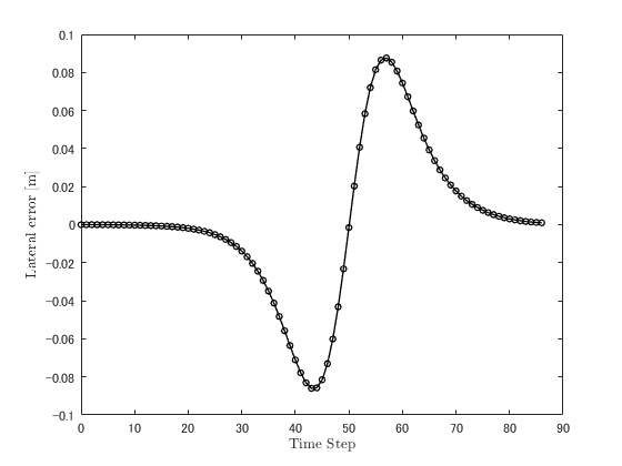
上記コードの実行結果を以下に示します.

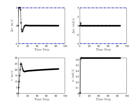

上記同様,軌道追従制御自体は出来ていますね. 最適制御問題の平均計算時間については,約0.0061秒と爆速で解いてますね(*゚∀゚)アヒャヒャ リアルタイム性に関しては全く問題ないですね!\(^o^)/
おわりに
今回は,モデル予測制御の最適制御問題を二次計画法で扱える形まで変形し,その効果を数値シミュレーションを通じて体感しました.少し数式をこねくり回して,二次計画法に帰着させるだけで,こんなに計算時間が向上するとは...
数学って本当大事だね( ´,_ゝ`)
参考文献
2.Vehicle Dynamics and Control, 2nd Edition
線形モデル予測制御入門:MATLABサンプルプログラム
目次
はじめに
前々から,気になっていたモデル予測制御ですが,以下の記事を見てさらに学習意欲が湧いたので記事にします.
上記の記事では,非線形モデル予測制御によりドリフト(横すべり)しながら障害物を回避する車両制御について書かれています.
トヨタは以前より,「うまい運転」を実現するために,モデル予測制御を取り入れていたようです.
記事の中では,こんな事が書かれています.
「制御においてMPCは可能性のある将来有望な手段と感じました。ただ、まだまだ小さな一歩でしかありません。これが製品になって実績ができてはじめて有効と判断できます。その意味でも、MPCを自動運転の制御に限らず、なんらかの形でアルゴリズムを世に出していければと考えています」(入江氏)
そういった意味では,今回のドリフト制御は大きな一歩を踏み出したと言えるのではないでしょうか!
さて,モデル予測制御については有識者の方々の素晴らしい記事が存在しています.
いまさら,私が記事にするのもおこがましい話ですが,備忘録としてまとめたいと思います. 前置きが長くなりましたが,次から本題に入ります.
モデル予測制御ってなに?
モデル予測制御とは,「制御対象の数式モデルを基に,制御周期ごとに最適制御問題を解くことで,未来の予測値から現時刻で取るべき制御入力を求める方法」です. モデル予測制御の概念図は以下の通りです.

モデル予測制御では図のように,制御周期(Sample Time)ごとに予測時間分(Prediction Horizon)の入力系列(Predicted Control Input)を計算します.ここでは,予測軌道(Predicted Output)が参照軌道(reference Trajectory)に追従するような入力系列を計算しています.実際に制御対象の入力として使われるのは,入力系列の最初の値になります.そして,時刻が遷移するたびに同様の流れで入力値を求めて制御していきます.やっていること自体は非常にシンプルなんです!
モデル予測制御における最適制御問題について
では,具体的に制御対象の数式モデルや最適制御問題はどのように表現されるのでしょうか? ますは,制御対象の数式モデルを定義します.
ここでは状態量、
は入力,
は出力です.
上記の方程式は,状態方程式と呼ばれるもので,現代制御理論で確立された表現です.
この制御モデルに基づき,最適制御問題は以下のように定式化されます.
ここで,はステージコスト,
は終端コストと呼ばれるものです.さらにNは考慮している予測時間の長さを表します.これらの具体的な数式は,制御対象や制御目的によって変動するため変数で置くことで一般化して表現しています.モデル予測制御では,毎時刻上記の最適制御問題を解くことで,現時刻で取るべき制御入力を算出しているのです!
数値シミュレーション
さて,数式だけ眺めていても具体的な作用や実装面でイメージがつかないため,ここでは簡単な例題を通じてモデル予測制御を体感してみましょう.
Case Study 1 : 倒立振子の姿勢制御
以下の方々の素晴らしい記事を参考に,モデル予測制御の数値シミュレーションをMATLABにより実装します.
制御対象の倒立振子の図を示します.

また,今回のシミュレーションではは0に近いという仮定を基に,線形近似した以下の数式モデルを制御対象とします.
ここで,状態量は4つあり,x方向の位置,x方向の速度,倒立振子の傾き角,倒立振子の傾き角速度で構成されます.
さらに,ステージコストと終端コストを以下のように設定します.
今回の制御目的は,全ての状態量が0に収束することとします.
下記が倒立振子制御のMATLABコードになります. また,ソルバーはYALMIPのIPOPTを使用しています.
clear;
close all;
clc;

%% Ipopt solver path
dir = pwd;
addpath(fullfile(dir,'Ipopt'))

%% Setup and Parameters
x0 = [-0.02; 0.0; 0.1; 0.0]; % Initial state of the inverted pendulum

dt = 0.1; % sample time
nx = 4;   % Number of states
nu = 1;   % Number of input

P = 30 * eye(nx);               % Termination cost weight matrix
Q = diag([1.0, 1.0, 1.0, 1.0]); % Weight matrix of state quantities
R = 0.01;                       % Weight matrix of input quantities
N = 10;                         % Predictive Horizon

% Range of states and inputs
xmin = [-5; -5; -5; -5];
xmax = [5; 5; 5; 5];
umin = -5;
umax = 5;

%% Linear Inverted Pendulum
M = 1.0;  % [kg]
m = 0.3;  % [kg]
g = 9.8;  % [m/s^2]
l = 2.0;  % [m]
system.dt = dt;
system.nx = nx;
system.nu = nu;
system.A = eye(nx) + [0.0, 1.0, 0.0, 0.0;
                      0.0, 0.0, m * g / M, 0.0;
                      0.0, 0.0, 0.0, 1.0;
                      0.0, 0.0, g * (M + m) / (l * M), 0.0] .* dt;
system.B = [0.0;
            1.0 / M;
            0.0;
            1.0 / (l * M)] .* dt;
system.xl = xmin;
system.xu = xmax;
system.ul = umin;
system.uu = umax;

%% MPC parameters
params_mpc.Q = Q;
params_mpc.R = R;
params_mpc.P = P;
params_mpc.N = N;

%% main loop
xTrue(:, 1) = x0;
uk(:, 1) = 0;
time = 20.0;
time_curr = 0.0;
current_step = 1;
solvetime = zeros(1, time / dt);

while time_curr <= time
    % update time
    time_curr = time_curr + system.dt;
    current_step = current_step + 1;

    % solve mac
    tic;
    uk(current_step)= mpc(xTrue(:, current_step - 1), system, params_mpc);
    solvetime(1, current_step - 1) = toc;

    % update state
    xTrue(:, current_step) = system.A * xTrue(:, current_step - 1) + system.B * uk(current_step);
end

%% solve average time
avg_time = sum(solvetime) / current_step;
disp(avg_time);

drow_figure(xTrue, uk, current_step);

%% model predictive control
function uopt = mpc(xTrue, system, params_mpc)
    % Solve MPC
    [feas, ~, u, ~] = solve_mpc(xTrue, system, params_mpc);
    if ~feas
        uopt = [];
        return
    else
        uopt = u(:,1);
    end
end

function [feas, xopt, uopt, Jopt] = solve_mpc(xTrue, system, params)
    % extract variables
    N = params.N;
    % define variables and cost
    x = sdpvar(system.nx, N+1);
    u = sdpvar(system.nu, N);
    constraints = [];
    cost = 0;

    % initial constraint
    constraints = [constraints; x(:,1) == xTrue];
    % add constraints and costs
    for i = 1:N
        constraints = [constraints;
            system.xl <= x(:,i) <= system.xu;
            system.ul <= u(:,i) <= system.uu
            x(:,i+1) == system.A * x(:,i) + system.B * u(:,i)];
        cost = cost + x(:,i)' * params.Q * x(:,i) + u(:,i)' * params.R * u(:,i);
    end
    % add terminal cost
    cost = cost + x(:,N+1)' * params.P * x(:,N+1);
    ops = sdpsettings('solver','ipopt','verbose',0);
    % solve optimization
    diagnostics = optimize(constraints, cost, ops);
    if diagnostics.problem == 0
        feas = true;
        xopt = value(x);
        uopt = value(u);
        Jopt = value(cost);
    else
        feas = false;
        xopt = [];
        uopt = [];
        Jopt = [];
    end
end

function drow_figure(xlog, ulog, current_step)
    % Plot simulation
    figure(1)
    subplot(2,2,1)
    plot(0:current_step - 1, xlog(1,:), 'ko-',...
        'LineWidth', 1.0, 'MarkerSize', 4);
    xlabel('Time Step','interpreter','latex','FontSize',10);
    ylabel('X[m]','interpreter','latex','FontSize',10);
    yline(0.0, '--r', 'LineWidth', 1.0);

    subplot(2,2,2)
    plot(0:current_step - 1, xlog(2,:), 'ko-',...
        'LineWidth', 1.0, 'MarkerSize', 4);
    xlabel('Time Step','interpreter','latex','FontSize',10);
    ylabel('$\dot{X}$[m/s]','interpreter','latex','FontSize',10);
    yline(0.0, '--r', 'LineWidth', 1.0);

    subplot(2,2,3)
    plot(0:current_step - 1, xlog(3,:), 'ko-',...
        'LineWidth', 1.0, 'MarkerSize', 4);
    xlabel('Time Step','interpreter','latex','FontSize',10);
    ylabel('$\theta$[rad]','interpreter','latex','FontSize',10);
    yline(0.0, '--r', 'LineWidth', 1.0);

    subplot(2,2,4)
    plot(0:current_step - 1, xlog(4,:), 'ko-',...
        'LineWidth', 1.0, 'MarkerSize', 4);
    xlabel('Time Step','interpreter','latex','FontSize',10);
    ylabel('$\dot{\theta}$[rad/s]','interpreter','latex','FontSize',10);
    yline(0.0, '--r', 'LineWidth', 1.0);

    figure(2)
    plot(0:current_step - 1, ulog(1,:), 'ko-',...
        'LineWidth', 1.0, 'MarkerSize', 4);
    xlabel('Time Step','interpreter','latex','FontSize',10);
    ylabel('Input F[N]','interpreter','latex','FontSize',10);
    yline(5.0, '--b', 'LineWidth', 2.0);
    yline(-5.0, '--b', 'LineWidth', 2.0);
end
https://github.com/Ramune6110/MATLAB_Robotics_Engineering/blob/main/Model_Predictive_Control/Linear_Model_Predictive_Control/Inverted_Pendulum.mgithub.com
上記コードの実行結果を以下に示します.


数値シミュレーション結果より,制御目的が達成されていることが確認できますね! ただし,予測ホライズンの長さやコストの重み行列の設定値によっては,きれいに収束しない場合もあります.そのため,モデル予測制御では,ある程度のパラメータ調整は必須と言えますね~.
また,最適制御問題の平均処理時間は約0.29sでした.平均処理時間についても,予測ホライズンの長さ,制御周期,最適化ソルバーによって変わるので一概に言えませんが,今回の結果に関して言えばリアルタイム性があるかどうかは微妙なところですかね~.倒立振子は割と不安定系なので,もう少し早く処理できるのが望ましいです.
Case Study 2 : 自動車の車線変更の制御
以下の資料を参考に,モデル予測制御の数値シミュレーションをMATLABにより実装します.
https://web.stanford.edu/class/archive/ee/ee392m/ee392m.1056/Lecture14_MPC.pdf
上記資料では,自動車の車両制御をモデル予測制御により実現しています.問題設定は以下の図の通りです.

ここでは,自動車は一定速度で走行しながらステアリング角度のみ制御することで,車線変更を実現するものとします.ステアリング角度の変動が微小だと仮定すると,自動車の縦方向の数理モデルは以下のように近似されます.
ここで,状態量は2つあり,縦方向のステアリング角速度,y方向の偏差で構成されます.
さらに,ステージコストと終端コストを以下のように設定します.
今回の制御目的は,へ追従することとします.
下記が車線変更の制御のMATLABコードになります.
clear;
close all;
clc;

%% Ipopt solver path
dir = pwd;
addpath(fullfile(dir,'Ipopt'))

%% Setup and Parameters
x0 = [0.0; 2.0]; % Initial state of the inverted pendulum

dt = 0.1;  % sample time
v  = 30.0; % driving speed
nx = 2;    % Number of states
nu = 1;    % Number of input

P = 30 * eye(nx);     % Termination cost weight matrix
Q = diag([1.0, 1.0]); % Weight matrix of state quantities
R = 0.01;             % Weight matrix of input quantities
N = 20;               % Predictive Horizon

% Range of states and inputs
xmin = [-5; -5];
xmax = [5; 5];
umin = -1;
umax = 1;

x_target = [0.0; 1.0]; % target state value

%% Linear Inverted Pendulum
system.dt = dt;
system.nx = nx;
system.nu = nu;
system.A = [1.0, 0.0;
            v * dt, 1.0];
system.B = [dt;
            0.5 * v * dt^2];
system.xl = xmin;
system.xu = xmax;
system.ul = umin;
system.uu = umax;

system.target = x_target;

%% MPC parameters
params_mpc.Q = Q;
params_mpc.R = R;
params_mpc.P = P;
params_mpc.N = N;

%% main loop
xTrue(:, 1) = x0;
uk(:, 1) = 0;
time = 1.0;
time_curr = 0.0;
current_step = 1;
solvetime = zeros(1, time / dt);

while time_curr <= time
    % update time
    time_curr = time_curr + system.dt;
    current_step = current_step + 1;

    % solve mac
    tic;
    uk(current_step) = mpc(xTrue(:, current_step - 1), system, params_mpc);
    solvetime(1, current_step - 1) = toc;

    % update state
    xTrue(:, current_step) = system.A * xTrue(:, current_step - 1) + system.B * uk(current_step);
end

%% solve average time
avg_time = sum(solvetime) / current_step;
disp(avg_time);

drow_figure(xTrue, uk, current_step);

%% model predictive control
function uopt = mpc(xTrue, system, params_mpc)
    % Solve MPC
    [feas, ~, u, ~] = solve_mpc(xTrue, system, params_mpc);
    if ~feas
        uopt = [];
        return
    else
        uopt = u(:,1);
    end
end

function [feas, xopt, uopt, Jopt] = solve_mpc(xTrue, system, params)
    % extract variables
    N = params.N;
    % define variables and cost
    x = sdpvar(system.nx, N+1);
    u = sdpvar(system.nu, N);
    constraints = [];
    cost = 0;

    % initial constraint
    constraints = [constraints; x(:,1) == xTrue];
    % add constraints and costs
    for i = 1:N
        constraints = [constraints;
            system.xl <= x(:,i) <= system.xu;
            system.ul <= u(:,i) <= system.uu
            x(:,i+1) == system.A * x(:,i) + system.B * u(:,i)];
        cost = cost + (x(:,i) - system.target)' * params.Q * (x(:,i) - system.target) + u(:,i)' * params.R * u(:,i);
    end
    % add terminal cost
    cost = cost + (x(:,N+1) - system.target)' * params.P * (x(:,N+1) - system.target);
    ops = sdpsettings('solver','ipopt','verbose',0);
    % solve optimization
    diagnostics = optimize(constraints, cost, ops);
    if diagnostics.problem == 0
        feas = true;
        xopt = value(x);
        uopt = value(u);
        Jopt = value(cost);
    else
        feas = false;
        xopt = [];
        uopt = [];
        Jopt = [];
    end
end

function drow_figure(xlog, ulog, current_step)
    % Plot simulation
    figure(1)
    subplot(2,1,1)
    plot(0:current_step - 1, xlog(1,:), 'ko-',...
        'LineWidth', 1.0, 'MarkerSize', 4);
    xlim([0, 11]);
    xlabel('Time Step','interpreter','latex','FontSize',10);
    ylabel('Heading angle[deg]','interpreter','latex','FontSize',10);
    yline(0.0, '--r', 'LineWidth', 1.0);

    subplot(2,1,2);
    plot(0:current_step - 1, xlog(2,:), 'ko-',...
        'LineWidth', 1.0, 'MarkerSize', 4);
    xlim([0, 11]);
    xlabel('Time Step','interpreter','latex','FontSize',10);
    ylabel('Lateral error[m]','interpreter','latex','FontSize',10);
    yline(1.0, '--r', 'LineWidth', 1.0);
    yline(1.5, '--k', 'LineWidth', 2.0);
    yline(2.5, 'k', 'LineWidth', 4.0);
    yline(0.5, 'k', 'LineWidth', 4.0);

    figure(2)
    plot(0:current_step - 1, ulog(1,:), 'ko-',...
        'LineWidth', 1.0, 'MarkerSize', 4);
    xlim([0, 11]);
    xlabel('Time Step','interpreter','latex','FontSize',10);
    ylabel('Steering input[deg/s]','interpreter','latex','FontSize',10);
    yline(1.0, '--b', 'LineWidth', 2.0);
    yline(-1.0, '--b', 'LineWidth', 2.0);
end
https://github.com/Ramune6110/MATLAB_Robotics_Engineering/blob/main/Model_Predictive_Control/Linear_Model_Predictive_Control/Lateral_Control_of_Car.mgithub.com
実は,倒立振子制御のコードとほとんど変わりません.変更箇所は,制御対象の数理モデル,ステージコストと終端コストぐらいです.
さらに,上記コードの実行結果を以下に示します.


数値シミュレーション結果より,きれいに車線変更できていることが確認できました!また,最適制御問題の平均処理時間は約0.38sでした.今回,予測ホライズンを20,制御周期を0.1sと設定したことに起因すると思います.が,自動車のようにリアルタイム性を求められる対象の制御としては,まだまだ改善する必要がありそうです...
Case Study 3 : 自動車の障害物回避
以下の論文の自動車モデルを参考に,自動車障害物回避のためのモデル予測制御の数値シミュレーションをMATLABにより実装します.
https://www.jstage.jst.go.jp/article/jacc/49/0/49_0_71/_pdf/-char/en
問題設定は以下の図の通りです.

ここでは,自動車の加速度,ステアリング角度を制御することで,静的障害物の回避制御をします. 今回の数値シミュレーションにおける最適制御問題を以下のように定義します.
さらに,ステージコストと終端コストを以下のように設定します.
注目すべきは,自車と障害物との距離が0以下にならないような制約を入れていることです.ただし,この制約はそのまま考慮するとハード制約となるため,今回はスラック変数を導出することで,制約条件を緩和(ソフト制約化)しています.ここで,スラック変数とは,ある程度の制約違反を許容する際に用いられる概念です.スラック変数の詳細については,式の記事が参考になります.
今回の制御目的は,障害物回避をしながら目的地へ到達することとします.
下記が自動車の障害物回避のMATLABコードになります.
clear;
close all;
clc;

%% Ipopt solver path
dir = pwd;
addpath(fullfile(dir,'Ipopt'))

%% Setup and Parameters
x0 = [0.0; 0.0; 0.0; 0.0; 0.0; 0.0]; % Initial state of the inverted pendulum

dt = 0.1; % sample time
nx = 6;   % Number of states
nu = 2;   % Number of input

P = 200 * eye(nx);                        % Termination cost weight matrix
Q = diag([1.0, 1.0, 1.0, 1.0, 1.0, 1.0]); % Weight matrix of state quantities
R = diag([0.1, 0.1]);                     % Weight matrix of input quantities
N = 10;                                   % Predictive Horizon
p = 200;                                  % salck weight value

% Range of states and inputs
xmin = [-5; -5; -5; -5; -5; -5];
xmax = [6; 6; 5; 5; 5; 5];
umin = [-1; -5];
umax = [1; 5];

% target state value
x_target = [6.0; 1.0; 0.0; 0.0; 0.0; 0.0];

% Obstacle
obs.pos = [3.0; 0.0];
obs.own_vehicle_diameter = 0.5; % [m]
obs.obstacle_diameter    = 0.5; % [m]
obs.r = obs.own_vehicle_diameter + obs.obstacle_diameter;

%% Linear Car models
M = 1500;     % [kg]
I = 2500;     % [kgm^2]
lf = 1.1;     % [m]
lr = 1.6;     % [m]
l = lf + lr;  % [m]
Kf = 55000;   % [N/rad]
Kr = 60000;   % [N/rad]
V = 20;       % [m/s]

system.dt = dt;
system.nx = nx;
system.nu = nu;

A53 = 2 * (Kf * lf + Kr * lr) / I;
A55 = -2 * (Kf * lf + Kr * lr) / (I * V);
A56 = -2 * (Kf * lf^2 + Kr * lr^2) / I;
A63 = 2 * (Kf + Kr) / M;
A65 = -2 * (Kf + Kr) / (M * V);
A66 = -2 * (Kf * lf + Kr * lr) / (M * V);
system.A = eye(nx) + [0.0, 0.0, 0.0, 1.0, 0.0, 0.0;
                      0.0, 0.0, 0.0, 0.0, 1.0, 0.0;
                      0.0, 0.0, 0.0, 0.0, 0.0, 1.0;
                      0.0, 0.0, 0.0, 0.0, 0.0, 0.0;
                      0.0, 0.0, A53, 0.0, A55, A56;
                      0.0, 0.0, A63, 0.0, A65, A66] .* dt;

B51 = 2 * Kf / M;
B61 = 2 * Kf * lf / I;
system.B = [0.0, 0.0;
            0.0, 0.0;
            0.0, 0.0;
            0.0, 1.0;
            B51, 0.0;
            B61, 0.0] .* dt;
system.xl = xmin;
system.xu = xmax;
system.ul = umin;
system.uu = umax;

system.target = x_target;

%% MPC parameters
params_mpc.Q = Q;
params_mpc.R = R;
params_mpc.P = P;
params_mpc.N = N;
params_mpc.p = p;

%% main loop
xTrue(:, 1) = x0;
uk(:, 1) = [0; 0];
time = 3.0;
time_curr = 0.0;
current_step = 1;
solvetime = zeros(1, time / dt);

while time_curr <= time
    % update time
    time_curr = time_curr + system.dt;
    current_step = current_step + 1;

    % solve mac
    tic;
    uk(:, current_step) = mpc(xTrue(:, current_step - 1), system, obs, params_mpc);
    solvetime(1, current_step - 1) = toc;

    % update state
    xTrue(:, current_step) = system.A * xTrue(:, current_step - 1) + system.B * uk(:, current_step);
end

%% solve average time
avg_time = sum(solvetime) / current_step;
disp(avg_time);

drow_figure(xTrue, uk, obs, x_target, current_step);

%% model predictive control
function uopt = mpc(xTrue, system, obs, params_mpc)
    % Solve MPC
    [feas, ~, u, ~] = solve_mpc(xTrue, system, obs, params_mpc);
    if ~feas
        uopt = [];
        return
    else
        uopt = u(:, 1);
    end
end

function [feas, xopt, uopt, Jopt] = solve_mpc(xTrue, system, obs, params)
    % extract variables
    N = params.N;
    % define variables and cost
    x = sdpvar(system.nx, N+1);
    u = sdpvar(system.nu, N);
    delta = sdpvar(1, N);
    constraints = [];
    cost = 0;

    % initial constraint
    constraints = [constraints; x(:,1) == xTrue];
    % add constraints and costs
    for i = 1:N
        constraints = [constraints;
            system.xl <= x(:,i) <= system.xu;
            system.ul <= u(:,i) <= system.uu
            x(:,i+1) == system.A * x(:,i) + system.B * u(:,i)];
        cost = cost + (x(:,i) - system.target)' * params.Q * (x(:,i) - system.target) + u(:,i)' * params.R * u(:,i);
    end
    % add collition avoidance constraints
    for i = 1:N
        pos = obs.pos;
        r = obs.r;
        distance = (x([1:2],i)-pos)'*((x([1:2],i)-pos)) - r^2;
        constraints = [constraints; distance >= delta(1, i)];
        cost = cost + delta(1, i)' * params.p * delta(1, i);
    end
    % add terminal cost
    cost = cost + (x(:,N+1) - system.target)' * params.P * (x(:,N+1) - system.target);
    ops = sdpsettings('solver','ipopt','verbose',0);
    % solve optimization
    diagnostics = optimize(constraints, cost, ops);
    if diagnostics.problem == 0
        feas = true;
        xopt = value(x);
        uopt = value(u);
        Jopt = value(cost);
    else
        feas = false;
        xopt = [];
        uopt = [];
        Jopt = [];
    end
end

function drow_figure(xlog, ulog, obs, x_target, current_step)
    % Plot simulation
    figure(1)
    subplot(2, 1, 1)
    plot(0:current_step - 1, ulog(1,:), 'ko-',...
        'LineWidth', 1.0, 'MarkerSize', 4);
    xlabel('Time Step','interpreter','latex','FontSize',10);
    ylabel('delta [rad]','interpreter','latex','FontSize',10);
    yline(1.0, '--b', 'LineWidth', 2.0);
    yline(-1.0, '--b', 'LineWidth', 2.0);

    subplot(2, 1, 2);
    plot(0:current_step - 1, ulog(2,:), 'ko-',...
        'LineWidth', 1.0, 'MarkerSize', 4);
    xlabel('Time Step','interpreter','latex','FontSize',10);
    ylabel('Acceleration [$m/s^2$]','interpreter','latex','FontSize',10);
    yline(5.0, '--b', 'LineWidth', 2.0);
    yline(-5.0, '--b', 'LineWidth', 2.0);

    figure(2)
    % plot trajectory
    plot(xlog(1,:), xlog(2,:), 'ko-',...
        'LineWidth', 1.0, 'MarkerSize', 4);
    hold on;
    grid on;
    axis equal;
    % plot initial position
    plot(xlog(1, 1), xlog(1, 2), 'dm', 'LineWidth', 2);
    % plot target position
    plot(x_target(1), x_target(2), 'dg', 'LineWidth', 2);
    xlabel('X[m]','interpreter','latex','FontSize',10);
    ylabel('Y[m]','interpreter','latex','FontSize',10);
    % plot obstacle
    pos = obs.pos;
    r = obs.obstacle_diameter;
    th = linspace(0,2*pi*100);
    x = cos(th);
    y = sin(th);
    plot(pos(1) + r*x, pos(2) + r*y, 'r', 'LineWidth', 2);
    plot(pos(1), pos(2), 'r', 'MarkerSize', 5, 'LineWidth', 2);
    % plot vegicle
    for i = 1:current_step
        r_vegicle = obs.own_vehicle_diameter;
        th = linspace(0,2*pi*100);
        x = cos(th);
        y = sin(th);
        X = xlog(1,i);
        Y = xlog(2,i);
        plot(X + r_vegicle * x, Y + r_vegicle * y, 'b','LineWidth', 2);
        hold on;
    end

    legend('Motion trajectory','Initial position', 'Target position','Obstacle', 'Location','southeast',...
           'interpreter','latex','FontSize',10.0);
end
https://github.com/Ramune6110/MATLAB_Robotics_Engineering/blob/main/Model_Predictive_Control/Linear_Model_Predictive_Control/Collision_Avoidance_of_Car.mgithub.com
倒立振子制御,自動車の車線変更制御のコードとの違いは,制御対象の数理モデル,制約条件,ステージコスト,終端コストです.
さらに,上記コードの実行結果を以下に示します.


数値シミュレーション結果より,きれいに障害物回避できていることが確認できました!しかし,最適制御問題の平均処理時間は約4.32sとかなり遅い結果となりました.予測ホライズンを10,制御周期0.1sに加え,スラック変数を導入したことで決定変数が増加したことが原因だと思います.車線変更制御同様,リアルタイム性の改善がまだまだ必要ですね><
おわりに
今回は,モデル予測制御の中でも最も基本の線形モデル予測制御について,数値例を示しながらまとめました.やはり,モデル予測制御の欠点である計算負荷が重いという問題が顕著に表れました.また,今回の数値例は比較的,線形モデルに近似しやすいものを扱いましたが,制御対象によってはそれが難しいことがあります.モデル予測制御は奥が深い~ (^-^)/.
参考文献
1.http://liu.diva-portal.org/smash/get/diva2:690771/FULLTEXT01.pdf